This article explores using data to uncover latent streams of returns, otherwise known as factors. We jump into the world of rotations to make sense of the factors and show how to ensure stability when used for real-world trading.
When you buy something and the price changes, what happened? Let’s say, for example, you buy shares in a made-up health company called “Orange.” This company makes wearable health monitors. The price of Orange goes down by 5%. Why? It could be because the whole market went down, or because the technology sector went down, or because the health sector went down, or because Orange genuinely performed poorly. Each of these possible explanations is called a factor.
The idea of a factor model is that every stream of returns can be explained by a number of underlying factors. A factor model roughly says $\boldsymbol{r}_t \approx \boldsymbol{L} \boldsymbol{f}_t$ where $\boldsymbol{r}_t$ is a vector of returns at time $t$, $\boldsymbol{L}$ is a matrix of factor loadings and $\boldsymbol{f}_t$ is a vector of factor returns. If we can identify these factors, we can understand what is driving returns.
Not only does this model allow us to explain returns, it lets us compare different assets in a meaningful way. For example, we can break down the returns of Apple and Orange and see how much of their returns are explained by the same factors.
There are a handful of ways to build a factor model. (1) You know the factors $\boldsymbol{f}_t$ and want to estimate the loadings $\boldsymbol{L}$. This is a macroeconomic factor model. (2) You know the loadings and you want to estimate the factors. This is a characteristic factor model. (3) You don’t know the factors or loadings and you want to estimate both. This is a statistical factor model1.
In this article, we’re going to explore statistical factor modeling. We will address a few issues that arise in this approach: (1) the method is data-hungry, requiring long historical return series; (2) the factors we get are often not economically meaningful; (3) the factors we get may not be stable out-of-sample.
Factor models
For a deep dive into factor models, the best resource on the market is The Elements of Quantitative Investing3. Here, we’ll lightly go over everything that will be useful for this article.
A factor model is formulated as
$$
\begin{equation}
\boldsymbol{r}_t = \boldsymbol{\alpha} + \boldsymbol{L} \boldsymbol{f}_t + \boldsymbol{\epsilon}_t \label{eq:factor_model}\tag{1}
\end{equation}
$$
where
$\boldsymbol{r}_t$ is a random vector of returns for $N$ assets at time $t$. Generally, the risk-free rate is subtracted, making these excess returns.
$\boldsymbol{\alpha}$ is the alpha vector. This is an $N \times 1$ vector of constants that represent the average return of each asset not explained by the factors.
$\boldsymbol{L}$ is the factor loading matrix. This is an $N \times K$ matrix where each row represents an asset and each column represents a factor. The entries represent the sensitivity of each asset to each factor.
$\boldsymbol{f}_t$ is a $K \times 1$ random vector of factor returns.
$\boldsymbol{\epsilon}_t$ is a random vector of idiosyncratic returns. This is an $N \times 1$ vector representing the portion of each asset’s return not explained by the factors.
The alpha vector $\boldsymbol{\alpha}$ is generally assumed to be $\text{E}[\boldsymbol{\alpha}] = 0$. If it is not, then we have an arbitrage opportunity. That is, we can find portfolio weights $\boldsymbol{w}$ such that $\boldsymbol{w}^\top \boldsymbol{\alpha} > 0$ and $\boldsymbol{w}^\top \boldsymbol{L} \boldsymbol{f}_t = 0$, meaning we can earn positive returns while having no exposure to the factors. In practice, a model that predicts asset returns is predicting this vector for time $t$, the elusive “alpha” that traders talk about.
Analogously, any model of $\text{E}[\boldsymbol{f}_t]$ is a model of the risk premia associated with each factor.
The ideal factor returns have a covariance matrix that is the identity matrix, i.e., $\boldsymbol{\Sigma}_f = \boldsymbol{I}$. The immediate implication of this is that the covariance of $\boldsymbol{r}_t$ is
$$
\boldsymbol{\Sigma}_r = \boldsymbol{L} \boldsymbol{\Sigma}_f \boldsymbol{L}^\top + \boldsymbol{\Sigma}_\epsilon = \boldsymbol{L} \boldsymbol{L}^\top + \boldsymbol{\Sigma}_\epsilon
$$
This condition turns out to be very easy to enforce as we will see later.
The idiosyncratic returns $\boldsymbol{\epsilon}_t$ are assumed to have expectation of 0 as any mean is captured with the $\boldsymbol{\alpha}$ vector. They are also assumed to be uncorrelated with the factors and generally with each other. This means that the covariance matrix $\boldsymbol{\Sigma}_\epsilon$ is a diagonal matrix. This is known as the idiosyncratic risk or specific risk of each asset. In practice, this assumption does not hold perfectly. Practitioners instead aim for a sparsely populated covariance matrix, meaning that most assets have little correlation with each other after accounting for the factors. Intuitively, if two assets are very similar, then they will have some correlation that is not explained by the factors.
Most factor models aim to have a small number of factors relative to the number of assets, $K \ll N$. For example, the commercially available MSCI USA Equity Factor Models factor models have on the order of 50-100 factors for 20,000+ assets. These factor models require vast data resources and research to build. They are expensive to purchase and used by large institutions.
For our purposes, we will focus on building a useful factor model that can be built with at-home resources. We will be using the same number of factors as assets, but we will still gain insight into the returns of our assets.
Why?
I said earlier that factor models allow us to explain returns. Why this is useful is not immediately obvious. Before we jump into the details of building these models, let’s explore what we can do with them.
You can explain where returns come from. By breaking down returns into alpha, factor and idiosyncratic returns, we can see what is driving portfolio returns. Say that our portfolio weights are $\boldsymbol{w}$ which means the portfolio return is $\boldsymbol{w}^\top \boldsymbol{r}_t$. Using the factor model in $\eqref{eq:factor_model}$, we can write the portfolio return as:
$$
\boldsymbol{w}^\top \boldsymbol{r}_t = \boldsymbol{w}^\top \boldsymbol{\alpha} + \boldsymbol{w}^\top \boldsymbol{L} \boldsymbol{f}_t + \boldsymbol{w}^\top \boldsymbol{\epsilon}_t
$$
where we can see exactly how much of the portfolio return is coming from each source.
You can explicitly model risk premia. Any model of the alpha vector $\boldsymbol{\alpha}$ is a model of the expected returns not explained by the factors. Any model of the factor returns $\boldsymbol{f}_t$ is a model of the risk premia associated with each factor. This means that if we have a model for $\text{E}[\boldsymbol{f}_t]$, we can directly trade on our beliefs about risk premia.
Additionally, any model of the asset returns $\text{E}[\boldsymbol{r}_t]$ can be decomposed into a model of $\boldsymbol{\alpha}$ and $\text{E}[\boldsymbol{f}_t]$. This decomposition allows us to understand whether our return predictions are coming from alpha or risk premia. This decomposition into alpha and factor returns is often called alpha orthogonal and alpha spanned respectively 3.
Build better risk models. Because we know where risks come from, we can hedge them. More specifically, we can invest in one or more factors while excluding others. These are factor-mimicking portfolios3.
You can build diversified portfolios. Rather than diversifying across assets which all share the same return drivers, you can directly diversify across factors. If the portfolio weights are $\boldsymbol{w}$, then the factor exposures are $\boldsymbol{w}^\top \boldsymbol{L}$. Therefore, you can choose portfolio weights $\boldsymbol{w}$ to achieve desired factor exposures.
Data
We’re going to use real data to illustrate the modeling in this article. We want a small selection of assets where we have long historical returns and that cover a wide range of the economy. To that end, we’ll use a selection of ETFs.
Choosing ETFs means we can focus on only a small number of assets but still capture a wide selection of the market. As ETFs tend to be mechanically constructed to track an index, we can extend their historical returns backwards by using either the index returns or the returns of related assets before the ETF was created.
In this article, we’re going to use the following U.S. ETFs:
At first, these ETFs look like they cover unrelated parts of the market. Looking at the figure below, we can see that the energy sector (XLE) is 45% correlated with the real estate sector (XLRE). In fact, all the ETFs are highly correlated, suggesting that there are similar underlying factors that they all share.
ETF correlation matrix. Shows the correlations between the selected ETFs over the period 2016-01-01 to 2025-11-25. The key thing to note is that all of the ETFs are highly correlated, suggesting that there are common factors driving their returns.
The only issue with these ETFs is that they have different inception dates and some only have a few years of history. For example, the communication services sector ETF (XLC) only has data from 2018 onward. To get around this, I construct synthetic returns for each ETF before its inception date, going back to 1990-01-01. I do this by getting a large set of related stock returns and index returns and regressing the first five years of ETF returns against these related returns. I then use the resulting regressed returns as the historical returns before the ETF’s inception date.
While this is not perfect, it does give us an approximation of the returns you might have realized if you were tracking the sector (or index) before the ETF was created.
The full details of this process are in the appendix.
As an example, here are the returns of the materials sector ETF (XLB) spliced onto the synthetic returns before inception:
Synthetic history example. The capital over time from investing in the materials sector ETF (XLB). From 1990-01-01 to 1998-12-15, the returns are synthetic, generated by regressing related stock and index returns against the actual ETF returns for the 5-year period starting at inception. After inception, the actual ETF returns are used. The synthetic returns after inception are included in the plot to show how well the synthetic returns approximate the actual returns after inception.
So that you can reproduce what we do here, the full set of returns can be downloaded here. You can read them in with:
Risk adjusting the returns to have a daily volatility of 1% and plotting the capital growth gives:
Statistical factors
Now that we have a long history of returns, we can build a statistical factor model. For this section, we are going to work in-sample. There are unique challenges when working out-of-sample that distract from the core modeling ideas. We will address these challenges later.
PCA
Principal component analysis (PCA) is the workhorse of statistical factor modeling. PCA transforms a dataset into a new set of orthogonal variables, called principal components, that are ordered by how much of the data’s variance they explain. This is achieved by rotating the coordinate system so that the first axis captures the largest possible spread in the data, the second captures the largest remaining spread subject to being independent of the first, and so on.
PCA is robust and deeply understood. Many before me have written excellent explanations of PCA, see for example this blog post. Here, we will go through the idea and the theory behind PCA as it relates to factor modeling.
Take $\boldsymbol{\Sigma}_r$ to be the $N \times N$ covariance matrix of asset returns. The set of orthonormal vectors ${\boldsymbol{p}_1, \boldsymbol{p}_2, \ldots, \boldsymbol{p}_N}$ that maximize the variance of the data projected onto them are the eigenvectors of $\boldsymbol{\Sigma}_r$. The variance explained by each vector is given by the corresponding eigenvalue ${\lambda_1, \lambda_2, \ldots, \lambda_N}$. We generally order the eigenvalues and corresponding eigenvectors in descending order $\lambda_1 \geq \lambda_2 \geq \ldots \geq \lambda_N$.
Collect the eigenvectors into a matrix:
$$
\boldsymbol{L}_\text{pca} = [\boldsymbol{p}_1, \boldsymbol{p}_2, \ldots, \boldsymbol{p}_N]
$$
Then, the factors at time $t$ are given by projecting the returns onto the eigenvectors:
$$
\boldsymbol{f}_t = \boldsymbol{L}_\text{pca}^\top \boldsymbol{r}_t
$$
and since the eigenvectors are orthonormal, the transpose is also the inverse $\boldsymbol{L}_\text{pca}\boldsymbol{L}_\text{pca}^\top = \boldsymbol{I}$. Thus, we have:
$$
\boldsymbol{r}_t = \boldsymbol{L}_\text{pca} \boldsymbol{f}_t
$$
which is a PCA factor model.
Rotating the data is a powerful idea that we will use repeatedly. For now, just note that we have not changed the data, simply rotated the coordinate system. The coordinate system we rotate into has useful properties that the original coordinate system did not have. In the case of PCA, the new coordinate system has uncorrelated axes ordered by variance.
The code to produce the PCA loadings and the inverse loadings (to convert returns to factors) looks like this:
defpca_loadings( cov: np.ndarray,)->tuple[np.ndarray, np.ndarray]:"""
Compute PCA factor loadings from a
covariance matrix.
Parameters
----------
cov : np.ndarray
Covariance matrix.
Returns
-------
loadings: np.ndarray
Factor loadings. Such that
r_t = L f_t
iloadings: np.ndarray
Inverse loadings. Such that
L^-1 r_t = f_t
""" eigvals, vecs = np.linalg.eigh(cov)# The eigenvalues and eigenvectors are# in ascending order. Reverse them so# that the largest eigenvalues are first. eigvals = eigvals[::-1] vecs = vecs[:,::-1] loadings = vecs
iloadings = vecs.T
return loadings, iloadings
Then to compute the factors from returns do:
cov = R.cov()_, iloadings = pca_loadings(cov)factors = R @ iloadings.T
You can check for yourself that the factors are not correlated by computing their correlation matrix: factors.corr().
Generally, when you run PCA, the idea is that you only keep the first $K$ factors that explain most of the variance. Previous work on factor modeling shows that there are on the order of 100 factors. In our case, we only have 14 assets, each of which covers a broad selection of the market. Therefore, I expect that all 14 factors are needed to explain the returns. So, we are going to keep all the factors.
Additionally, by keeping all the factors, $\boldsymbol{L}_\text{pca}$ is square and invertible, which means we lose the terms $\boldsymbol{\alpha}$ and $\boldsymbol{\epsilon}_t$ from the factor model:
$$
\boldsymbol{r}_t = \boldsymbol{L}_\text{pca} \boldsymbol{f}_t
$$
The returns can be perfectly reconstructed from the factors and vice versa.
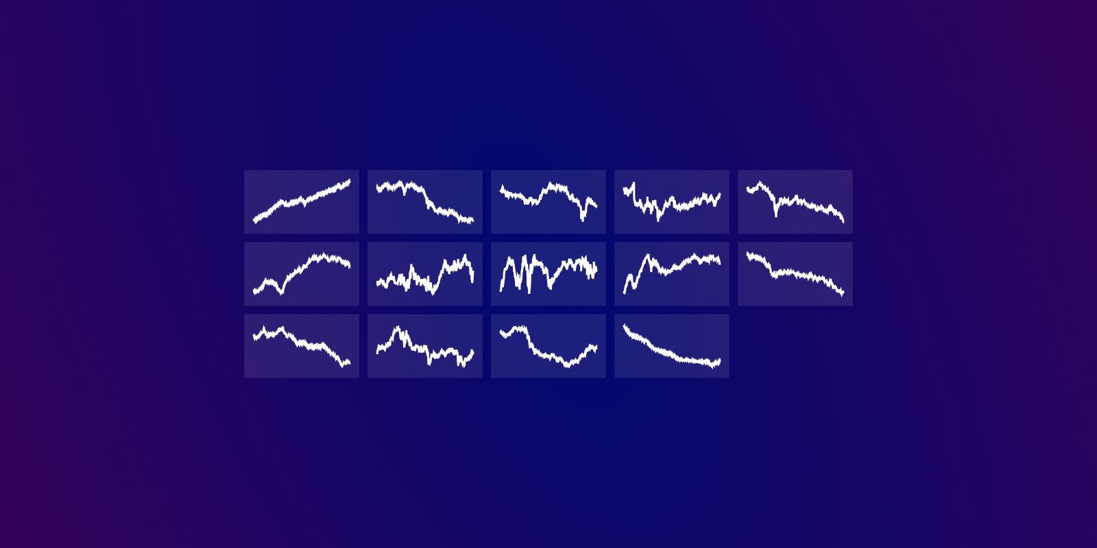
We can visualize the factors by adjusting their volatilities to be 1% per day. This dampens out the extreme movements when calculating the capital growth for each factor. The factors look like:
The first factor is often called the “market factor” as it tends to represent the overall market movement. As we are looking at equities, we could interpret the first factor as the equity risk premia. That is, this is the return that investors expect to earn for taking on equity risk.
The big question is: What do the other factors represent economically? We’ve found orthogonal streams of returns, but besides the market factor, do the other factors represent anything meaningful? Without some understanding of what the factors are, we will struggle (emotionally) to allocate capital to them—particularly during times of crisis.
The only data we have are the ETF returns. If a factor explains a large portion of a particular sector and very little of the others, we can say that the factor represents the stream of returns for that sector. We can do this by looking at the loadings matrix $\boldsymbol{L}_\text{pca}$. However, because each factor has different variance, the loadings are not comparable.
To solve this, we whiten the factors.
Whitening
The idea behind whitening is to rescale the factors to have the same variance. Generally, we set the variance to 1. The factors are already uncorrelated, which means that setting their variances makes their covariance matrix the identity matrix.
To whiten, we divide the factors by their standard deviations. The eigenvalues from PCA are the variances of each factor. Therefore, we can whiten by dividing each factor by the square root of its corresponding eigenvalue.
Set $\boldsymbol{D}$ to be a diagonal matrix where each entry is $D_{ii} = \sqrt{\lambda_i}$. Then, we can write the whitened factor model as:
$$
\begin{aligned}
\boldsymbol{f}_t &= \boldsymbol{D}^{-1}\boldsymbol{L}_\text{pca}^\top \boldsymbol{r}_t \\
\\
\boldsymbol{r}_t &= \boldsymbol{L}_\text{pca}\boldsymbol{D} \boldsymbol{f}_t \\
\end{aligned}
$$
And the loadings and inverse loadings become:
$$
\begin{aligned}
\boldsymbol{L} &= \boldsymbol{L}_\text{pca}\boldsymbol{D} \\
\boldsymbol{L}^{-1} &= \boldsymbol{D}^{-1}\boldsymbol{L}_\text{pca}^\top \\
\end{aligned}
$$
The PCA loadings function is updated with:
defpca_loadings( cov: np.ndarray, whiten:bool=False,)->tuple[np.ndarray, np.ndarray]:...# Existing codeif whiten:# Whiten loadings so that the factors have# covariance = I seigvals = np.sqrt(eigvals)[:,None]# Column vector loadings = loadings * seigvals.T
iloadings =(1/ seigvals)* iloadings
return loadings, iloadings
The whitened factors all have unit variance and are uncorrelated. This means that the covariance matrix of the factors is the identity matrix:
$$
\boldsymbol{\Sigma}_f = \text{Cov}[\boldsymbol{f}_t] = \boldsymbol{I}
$$
As the factors are now statistically the same, we can compare the loadings. We specifically want to know how much of each asset’s variance is explained by each factor. The covariance matrix of returns under our factor model is:
$$
\boldsymbol{\Sigma}_r = \text{Cov}[\boldsymbol{r}_t] = \boldsymbol{L} \text{Cov}[\boldsymbol{f}_t] \boldsymbol{L}^\top = \boldsymbol{L} \boldsymbol{I} \boldsymbol{L}^\top = \boldsymbol{L} \boldsymbol{L}^\top
$$
where the variance of asset $i$ is the $i$th diagonal entry of $\boldsymbol{\Sigma}_r$:
$$
\sigma^2_{r,i} = \sum_{j=1}^K L_{ij}^2
$$
that sum of squared loadings is the sum over the row of $\boldsymbol{L}$ corresponding to asset $i$. The value $L_{ij}^2$ is the contribution of factor $j$ to the variance of asset $i$.
We’re going to define the contribution matrix as the matrix $\boldsymbol{C}$ where each entry is the proportion of asset $i$’s variance explained by factor $j$, with the sign added back in:
$$
C_{ij} = \frac{L_{ij}^2}{\sigma^2_{r,i}} = \text{sign}(L_{ij}) \frac{L_{ij}^2}{\sum_{k=1}^K L_{ik}^2}
$$
We say that factor $j$ contributes $C_{ij}$ percent to asset $i$’s variance. Note that the absolute contributions for each asset sum to 1. We keep the sign to help with interpretation later. The code to compute the contribution matrix is:
We can then visualize the contribution matrix by plotting the contributions by factor:
We can make the following observations from the contribution matrix:
Market factor. The first factor is very clearly the market factor. It explains most of the variance for each of the assets.
Inexplicable factors. Most of the remaining factors do not explain a small set of assets. For example, see factor 2. Instead, they appear to explain similar proportions of many assets.
Explainable factors. A couple of factors do appear to have some meaning. For example, factor 4 explains a much larger proportion of utilities (XLU) than the other assets. We could say that this factor represents the utilities sector.
Decreasing explaining power. As we go to higher numbered factors, the amount of variance explained decreases. This is expected as PCA orders the factors by variance explained.
The conclusion so far is that besides the first factor, the remaining factors have no clear economic meaning. We can get around this by noting that we do not care that the PCA factors represent directions of maximum variance. We only care that they are uncorrelated. Therefore, we can rotate the factors out of the PCA coordinate system into another coordinate system that is more interpretable.
Rotations
Recall that the PCA loadings are simply a rotation of the returns into a new coordinate system with special properties. Now that we’ve whitened the factors, rotations become very powerful.
A rotation is represented by an orthonormal matrix $\boldsymbol{G}$ where:
$$
\boldsymbol{G}^\top \boldsymbol{G} = \boldsymbol{G} \boldsymbol{G}^\top = \boldsymbol{I}
$$
which means that we can rotate the factors by any valid rotation matrix without changing the model:
$$
\boldsymbol{r}_t = \boldsymbol{L} \boldsymbol{f}_t = \boldsymbol{L} \boldsymbol{G} \boldsymbol{G}^\top \boldsymbol{f}_t
$$
The rotated factors are $ \boldsymbol{G}^\top \boldsymbol{f}_t$ and critically:
$$
\text{Cov}[\boldsymbol{G}^\top \boldsymbol{f}_t] = \boldsymbol{G}^\top \text{Cov}[\boldsymbol{f}_t] \boldsymbol{G} = \boldsymbol{G}^\top \boldsymbol{I} \boldsymbol{G} = \boldsymbol{I} = \text{Cov}[\boldsymbol{f}_t]
$$
So any valid rotation matrix maintains the orthonormality of the factors! This is powerful because it means we can search for a rotation matrix that makes the factors more interpretable while still maintaining the properties we want.
We’re going to look at a rotation that makes the factors more interpretable—the varimax rotation.
Varimax rotation
We can make the factors more interpretable by making the loadings matrix $\boldsymbol{L}$ sparser. That is, for each factor (column of $\boldsymbol{L}$), we want only a few assets to have large loadings, and the rest to be close to zero. This makes it easy to interpret what each factor is doing, as it only strongly influences a few assets. One rotation that achieves this is called the varimax rotation, first described in 1958 in psychometric research 4.
Note again that the covariance matrix of returns under our factor model with orthonormal factors is:
$$
\boldsymbol{\Sigma}_r = \boldsymbol{L} \boldsymbol{L}^\top
$$
where the variance of asset $i$ is the $i$th diagonal entry of $\boldsymbol{\Sigma}_r$:
$$
\sigma^2_{r,i} = \sum_{j=1}^K L_{ij}^2
$$
That sum of squared loadings is the sum over the row of $\boldsymbol{L}$ corresponding to asset $i$. We previously named the value $L_{ij}^2$ the contribution of factor $j$ to the variance of asset $i$. If we want each factor to contribute to only a few assets, we want the squared loadings in each column of $\boldsymbol{L}$ to be sparse.
We can formulate this sparsity requirement by saying we want each column of $\boldsymbol{L}$ to have a high variance of squared loadings. If the squared loadings are all similar, then the variance is low. If some squared loadings are large and the rest are small, then the variance is high. Recall that the variance of a random variable $X$ is given by $\text{Var}(X) = \text{E}[X^2] - (\text{E}[X])^2$. Therefore, the variance of the squared loadings for factor $j$ is:
And the varimax objective function to maximize is the sum of these variances across all factors:
$$
\text{Varimax}(\boldsymbol{L}) = \sum_{j=1}^K \left[ \frac{1}{N} \sum_{i=1}^N L_{ij}^4 - \left( \frac{1}{N} \sum_{i=1}^N L_{ij}^2 \right)^2 \right]
$$
The original solution to maximizing this objective rotates a single pair of factors at a time to increase the objective 4. The modern approach is to calculate the gradient and use an iterative method to find the maximum 5. We’ll skip the derivation and just present the algorithm. Say that the given unrotated loadings matrix is $\boldsymbol{L} = \boldsymbol{L}_\text{pca}\boldsymbol{D}$. The algorithm is:
Initialize the rotation $\boldsymbol{G} \leftarrow \boldsymbol{I}$.
Compute column means $d_j = \tfrac{1}{p}\sum_i \Lambda_{ij}^2$.
Compute the derivative $\partial \text{Varimax}(\boldsymbol{L})/\partial\boldsymbol{\Lambda} = \tfrac{4}{p}\boldsymbol{Z}$ where the entries are $Z_{ij} = \Lambda_{ij}^3 - d_j \Lambda_{ij}$.
Using the chain rule, compute the derivative $\boldsymbol{M} = \partial \text{Varimax}(\boldsymbol{L})/\partial \boldsymbol{G} = \boldsymbol{L}^\top \boldsymbol{Z}$.
Compute the SVD: $\boldsymbol{M} = \boldsymbol{U} \boldsymbol{\Sigma} \boldsymbol{V}^\top$.
If the objective has not converged, go back to step 2.
The code for the varimax algorithm in Python is:
defvarimax_rotation( loadings: np.ndarray, max_iter:int=1000, tol:float=1e-5,)-> np.ndarray:"""
Calculates the varimax rotation matrix
corresponding to the input loading matrix.
Code is stolen and modified from the
factor_analyzer package.
Parameters
----------
loadings : array-like
The loading matrix.
max_iter : int, optional
The maximum number of iterations.
Defaults to 1000.
tol : float, optional
The convergence threshold.
Defaults to 1e-5.
Returns
-------
rotation_mtx : array-like
The rotation matrix. The loadings
are rotated by: L @ rotation_mtx
""" X = loadings.copy() n_rows, n_cols = X.shape
if n_cols <2:return X
# initialize the rotation matrix# to N x N identity matrix rotation_mtx = np.eye(n_cols) d =0for _ inrange(max_iter): old_d = d
# take inner product of loading matrix# and rotation matrix basis = np.dot(X, rotation_mtx)# transform data for singular value decomposition using updated formula :# B <- t(x) %*% (z^3 - z %*% diag(drop(rep(1, p) %*% z^2))/p) diagonal = np.diag(np.squeeze(np.repeat(1, n_rows).dot(basis**2))) transformed = X.T.dot(basis**3- basis.dot(diagonal)/ n_rows)# perform SVD on# the transformed matrix U, S, V = np.linalg.svd(transformed)# take inner product of U and V, and sum of S rotation_mtx = np.dot(U, V) d = np.sum(S)# check convergenceif d < old_d *(1+ tol):breakreturn rotation_mtx
For our analysis, we’re going to make a small change to the algorithm. The first factor we found with PCA is the market factor. Recall that the loadings for that factor are all fairly even. If we were to use the varimax rotation, we would lose this factor, as varimax does not favor factors with even loadings. We want to hold this factor fixed and only rotate the other factors. We pull this off by excluding the column in $\boldsymbol{L}$ corresponding to the market factor when computing the varimax rotation. That is, we run varimax on $\boldsymbol{L}_{2:K}$, and then the rotation matrix is:
$$
\boldsymbol{G} = \begin{bmatrix}1 & \boldsymbol{0} \\
\boldsymbol{0} & \boldsymbol{G}_{varimax} \\
\end{bmatrix}
$$
The final step we want to do is ensure that the factors have a consistent sign. PCA has an indeterminacy where the sign of each factor is arbitrary. We will fix the sign by ensuring that the largest contribution for each factor is positive. This amounts to a diagonal matrix $\boldsymbol{S}$ where $S_{ii} = \pm 1$, depending on the sign of the largest contribution for factor $i$. $\boldsymbol{S}$ is orthonormal, and thus it is a valid rotation matrix. We’ll use the following function to get the sign matrix:
defsign_rotation(loadings: np.ndarray)-> np.ndarray: c = contribution_matrix(loadings) signs = np.sign([max(c[:, j], key=abs)for j inrange(c.shape[1])]) signs[signs ==0]=1# avoid zeros S = np.diag(signs)return S
Our factor model with PCA, whitening, varimax rotation and sign consistency becomes:
$$
\begin{aligned}
\boldsymbol{f}_t &= \boldsymbol{S}^\top \boldsymbol{G}^\top \boldsymbol{D}^{-1}\boldsymbol{L}_\text{pca}^\top \boldsymbol{r}_t \\
\\
\boldsymbol{r}_t &= \boldsymbol{L}_\text{pca}\boldsymbol{D} \boldsymbol{G} \boldsymbol{S} \boldsymbol{f}_t \\
\end{aligned}
$$
and you can compute everything with:
cov = R.cov()loadings, iloadings = pca_loadings(cov, whiten=True)# Varimax rotate all but the first (market) factorG = np.eye(loadings.shape[1])G[1:,1:]= varimax_rotation(loadings[:,1:])loadings = loadings @ G
iloadings = G.T @ iloadings
# Make sure everything is positiveS = sign_rotation(loadings)loadings = loadings @ S
iloadings = S @ iloadings
Interpretation
Our process for finding factors is: obtain PCA factors, whiten them, varimax rotate all but the first factor, and ensure positive signs. We then convert the loadings matrix to the contribution matrix for interpretation as before.
The results look like:
These results are quite remarkable.
In comparison to the unrotated PCA factors, the varimax factors are much more interpretable. Factor 1 remains the market factor with all assets contributing fairly evenly. The other factors have become much more sparse. Keep in mind that these factors are all uncorrelated! So a factor that explains a high percentage of one asset and little of the others can be thought of as the unique source of risk and returns for that asset.
Factor 1 is the market factor. This explains a high percentage of all assets, roughly 50% for each asset. Factor 4 explains a high percentage of the utilities sector (XLU). There is some explaining power for other ETFs, but it is tiny in comparison. We should expect to see small explaining power for all the other ETFs as the sectors economically overlap. If Factor 4 has a positive average return, then it could be interpreted as the utilities sector risk premia. Each factor in our example explains a high percentage of one of the assets and thus similar conclusions can be drawn for the other factors.
The logged factor returns look like:
At this point, we could talk about how to model the possible risk premia in each factor. We will leave that to another article. Instead, we will look at ensuring that a factor model maintains its properties out-of-sample.
In practice
Up until now, the factor modeling has operated in-sample. That is, we have looked at factors historically computed with all available data. In practice, we want to be able to compute factor loadings and factors out-of-sample. That is, at time $t$, we want to be able to compute the factor loadings $\boldsymbol{\beta}$ using data available before time $t$ and factors $\boldsymbol{f}_t$ using only data available up to time $t$.
We’re now going to switch from a fixed matrix of loadings $\boldsymbol{L}$ to time varying loadings $\boldsymbol{L}_t$. For factors at time $t$, we will compute the loadings using data up to time $t-l$ where $l$ is a suitable lag. The factor model becomes:
$$
\boldsymbol{r}_t =\boldsymbol{\alpha} + \boldsymbol{L}_{t-l} \boldsymbol{f}_t + \boldsymbol{\epsilon}_t
$$
We will assume that $\boldsymbol{\alpha} = 0$ and we will use a cross-sectional regression to compute the factor returns once the asset returns are realized:
$$
\boldsymbol{f}_t = (\boldsymbol{L}_{t-l}^\top \boldsymbol{L}_{t-l})^{-1} \boldsymbol{L}_{t-l}^\top \boldsymbol{r}_t
$$
Because our loadings are invertible, this gives us the exact factor returns that reconstruct the realized returns:
$$
\boldsymbol{r}_t = \boldsymbol{L}_{t-l} \boldsymbol{f}_t
$$
Exponential weighting
When computing the covariance matrix of returns to fit the PCA factor model, we could use a sliding window of historical returns. This approach gives equal weight to all returns in the window and zero weight to returns outside the window. A better approach is to use an exponentially weighted moving covariance matrix. This approach gives more weight to recent returns and less weight to older returns.
We have a whole article on the exponentially weighted variance here. In Python, we can compute the exponentially weighted covariance matrix with:
When computing the factor loadings at time $t$, we use the exponentially weighted covariance matrix up to time $t-l$.
Loadings consistency
Both the PCA and varimax rotations do not have unique solutions. This means that when we compute the loadings day to day, the loadings may change in ways that make them impossible to interpret consistently over time.
PCA has an indeterminacy where the sign of each factor is arbitrary. See the figure below. This means that if we compute the loadings at different times, the signs of the factors may be flipped. This means that the factors will flip signs randomly day to day, making them impossible to interpret.
Example of PCA indeterminacy. The sign of the PCA factors is arbitrary. Here we illustrate two possible PCA factorizations of the same data. The difference is that the signs of the factors have been flipped. Both factorizations are equally valid PCA decompositions.
The varimax rotation is an optimization over a non-convex objective. There are many solutions and local minima. Consider that since the factors are whitened, the order of the factors is not important. In fact, the same factors can be represented in any order, which immediately gives us $K!$ equivalent solutions. This means that the factors will change meaning day to day, making them impossible to interpret consistently out-of-sample.
For example, we’ll fit our factor model to a moving EWM covariance matrix with a half-life of $252 \times 2$ days. We’ll calculate the contributions matrix and plot the contributions for the 2nd factor over time. You can see the results in the figure below, which shows that the contributions are all over the place:
Example of rotation indeterminacy. The contributions of the 2nd factor over time are shown. The factor model was fitted with an EWM covariance matrix with a half-life of two years. You can observe that the contributions (and thereby the factor loadings) change meaning significantly over time.
We can solve this by computing the loadings for time $t+1$ and rotating them to be as close as possible to the previous day’s loadings. This means we want an orthonormal matrix $\boldsymbol{Q}$ such that the rotated loadings $\boldsymbol{L}_{t+1} \boldsymbol{Q}$ are as close as possible to the previous day’s loadings $\boldsymbol{L}_t$. We can formulate this as the minimization problem:
$$
\begin{aligned}
\arg\min_{\boldsymbol{Q}} & \ || \boldsymbol{L}_{t+1} \boldsymbol{Q} - \boldsymbol{L}_t ||_F^2 \\
\text{s.t.} & \ \boldsymbol{Q}^\top \boldsymbol{Q} = \boldsymbol{I} \\
\end{aligned}
$$
This is known as the orthogonal Procrustes problem and has a closed-form solution. The derivation of the solution is in the appendix. We’ll just present the final result here. The solution is to take the following SVD:
$$
\boldsymbol{L}_t^\top \boldsymbol{L}_{t+1} = \boldsymbol{U} \boldsymbol{\Sigma} \boldsymbol{V}^\top
$$
and solve:
$$
\boldsymbol{Q} = \boldsymbol{U} \boldsymbol{V}^\top
$$
The code to implement this rotation matrix is:
defprocrustes_rotation(current, previous): C = previous.T @ current
U, _, Vt = np.linalg.svd(C) Q = Vt.T @ U.T
return Q
Repeating the analysis from before, we can examine the contributions of the 2nd factor over time after applying the Procrustes rotation each day:
Example of rotation indeterminacy fixed with Procrustes rotation. The contributions of the 2nd factor over time are shown. The factor model was fitted with an EWM covariance matrix with a half-life of two years. Additionally, the Procrustes rotation was applied each day to ensure that the loadings remain consistent over time. You can observe that the contributions (and thereby the factor loadings) are now stable over time.
Factor orthogonality
Because the loadings are changing over time, the factors we get may not be orthonormal. That is, the covariance matrix of the factors may not be the identity matrix:
$$
\boldsymbol{\Sigma}_f = \text{Cov}[\boldsymbol{f}_t] \neq \boldsymbol{I}
$$
There is no way to fix this. We can reduce the issue by further rotating the factors at each time step. However, this further rotation impacts the interpretability of the factors and in my experience, only marginally improves the orthogonality of the factors.
For now, we will accept that the factors are not perfectly orthonormal out-of-sample. We still have a significantly improved stream of returns. Recall the correlation matrix of the ETF returns from before. Now, observe the correlation matrix of the factor returns:
Factor correlation matrix. Shows the correlations between the realized factor returns over the period 2016-01-01 to 2025-11-25. In comparison to the ETF correlation matrix, the factors are mostly uncorrelated, showing that the factor model has successfully identified sources of risk and return.
In comparison to the ETF correlation matrix, the factors are mostly uncorrelated. There are some clusters of small correlations; factor 14 has some negative correlations with a bunch of the factors. However, the level of correlations is tiny in comparison to the raw ETF returns. We can easily conclude that the factor model has successfully identified sources of risk and return.
Interpretation
Now that we’ve stabilized the out-of-sample factor model, we can inspect the factors over time to check that they are in fact stable and interpretable. For each factor, we’ll plot the contributions over time for each of the assets:
I’ve omitted the names of each asset/line to keep the figure clean. The main point is that the factors maintain their meaning over time. This is exactly what we wanted. Each factor represents a unique source of risk and return and it is stable out-of-sample.
For the curious, here are the logged factor returns over time:
You can replicate this analysis with the following code:
This article builds a practical statistical factor model for ETF returns that is interpretable and stable out-of-sample. The model uses PCA as a starting point and then applies a series of rotations to force interpretability and stability. The resulting factors are mostly uncorrelated and represent economically meaningful sources of risk and return.
To be able to examine the long-term behavior of the factors, long-run historical returns were approximated for each of the assets.
You can apply this method to any set of asset returns where you have enough historical data. The methods are not limited to ETFs, nor to a daily frequency. The key steps are:
Collect historical returns for your assets.
Compute an exponentially weighted covariance matrix of returns.
Compute PCA loadings and whiten the factors.
Apply a varimax rotation (holding the market factor fixed).
Apply a sign-consistency rotation.
For out-of-sample, apply a Procrustes rotation to ensure stability.
The selection of ETFs covers three market indexes (S&P 500, NASDAQ-100, and Russell 2000) and the U.S. sector indexes.
We want to extend the ETF returns back to 1990-01-01. To do this, we:
Construct a list of Yahoo Finance tickers of instruments that were trading from 1990-01-01 to now.
Download the daily returns for these instruments from Yahoo Finance.
For each ETF, take the first 5 years of returns and regress the ETF returns on the returns of the instruments in the dataset from step 2.
Use the regression coefficients to construct synthetic returns for the ETFs going back to 1990-01-01.
To construct the list of tickers, I downloaded the list of current holdings for each of the ETFs. For example, you can find an Excel document of holdings for XLK on this page. I then limited this list to instruments that were trading from 1990-01-01 to now. I also added the following indexes to the list:
Given two matrices of the same shape $\boldsymbol{L}_{t+1}$ and $\boldsymbol{L}_{t}$ the orthogonal Procrustes problem is:
$$
\begin{aligned}
\boldsymbol{Q}^* &= \arg\min_{\boldsymbol{Q}} || \boldsymbol{L}_{t+1} \boldsymbol{Q} - \boldsymbol{L}_t ||_F^2 \\
\text{s.t.} & \ \boldsymbol{Q}^\top \boldsymbol{Q} = \boldsymbol{I} \\
\end{aligned}
$$
This is known as the orthogonal Procrustes problem and has a closed form solution. The Frobenius norm can be written as a trace:
$$
|| \boldsymbol{L}_{t+1} \boldsymbol{Q} - \boldsymbol{L}_t ||_F^2 =
\text{Tr} \left((\boldsymbol{L}_{t+1} \boldsymbol{Q} - \boldsymbol{L}_t)^\top (\boldsymbol{L}_{t+1} \boldsymbol{Q} - \boldsymbol{L}_t)\right)
$$
expanding out the trace gives:
$$
= \text{Tr}(\boldsymbol{Q}^\top \boldsymbol{L}_{t+1}^\top \boldsymbol{L}_{t+1} \boldsymbol{Q}) - 2 \text{Tr}(\boldsymbol{L}_t^\top \boldsymbol{L}_{t+1} \boldsymbol{Q}) + \text{Tr}(\boldsymbol{L}_t^\top \boldsymbol{L}_t)
$$
We can use the cyclic property of traces to rewrite the first term:
$$
\text{Tr}(\boldsymbol{Q}^\top \boldsymbol{L}_{t+1}^\top \boldsymbol{L}_{t+1} \boldsymbol{Q}) = \text{Tr}(\boldsymbol{Q}\boldsymbol{Q}^\top \boldsymbol{L}_{t+1}^\top \boldsymbol{L}_{t+1})
$$
and since $\boldsymbol{Q}$ is orthonormal, $\boldsymbol{Q}\boldsymbol{Q}^\top = \boldsymbol{I}$. Therefore, the first term is constant with respect to $\boldsymbol{Q}$. The third term is also constant with respect to $\boldsymbol{Q}$. Therefore, the only $\boldsymbol{Q}$ dependent term is the middle term:
$$
|| \boldsymbol{L}_{t+1} \boldsymbol{Q} - \boldsymbol{L}_t ||_F^2 = \text{const} - 2 \text{Tr}(\boldsymbol{L}_t^\top \boldsymbol{L}_{t+1} \boldsymbol{Q})
$$
Now, minimizing the Frobenius norm is equivalent to:
$$
\begin{aligned}
\boldsymbol{Q}^* &= \arg\max_{\boldsymbol{Q}} \ \text{Tr}(\boldsymbol{L}_t^\top \boldsymbol{L}_{t+1} \boldsymbol{Q}) \\
\text{s.t.} & \ \boldsymbol{Q}^\top \boldsymbol{Q} = \boldsymbol{I} \\
\end{aligned}
$$
Now set $\boldsymbol{C} = \boldsymbol{L}_t^\top \boldsymbol{L}_{t+1}$ and take the SVD of $\boldsymbol{C} = \boldsymbol{U} \boldsymbol{\Sigma} \boldsymbol{V}^\top$:
$$
\boldsymbol{C} = \boldsymbol{U} \boldsymbol{\Sigma} \boldsymbol{V}^\top
$$
The problem then becomes:
$$
\begin{aligned}
\boldsymbol{Q}^* &= \arg\max_{\boldsymbol{Q}} \ \text{Tr}(\boldsymbol{U} \boldsymbol{\Sigma} \boldsymbol{V}^\top \boldsymbol{Q}) \\
\text{s.t.} & \ \boldsymbol{Q}^\top \boldsymbol{Q} = \boldsymbol{I} \\
\end{aligned}
$$
Using the cyclic property of traces again gives:
$$
= \text{Tr}(\boldsymbol{\Sigma} \boldsymbol{V}^\top \boldsymbol{Q} \boldsymbol{U})
$$
Now, let $\boldsymbol{W} = \boldsymbol{V}^\top \boldsymbol{Q} \boldsymbol{U}$ and write:
$$
\text{Tr}(\boldsymbol{\Sigma} \boldsymbol{W}) = \sum_{i=1}^K \sigma_i W_{ii}
$$
where $\sigma_i$ are the diagonal entries of $\boldsymbol{\Sigma}$.
Since $\boldsymbol{Q}$, $\boldsymbol{U}$, and $\boldsymbol{V}$ are all orthonormal, $\boldsymbol{W}$ is also orthonormal. This means that the entries of $\boldsymbol{W}$ are bounded by $|W_{ij}| \leq 1$. Since the singular values $\sigma_i$ are non-negative, we can maximize the trace by setting $W_{ii} = 1$ for all $i$. If the diagonal entries of $\boldsymbol{W}$ are all 1, and the matrix is orthonormal, then $\boldsymbol{W} = \boldsymbol{I}$. Therefore:
$$
\boldsymbol{V}^\top \boldsymbol{Q} \boldsymbol{U} = \boldsymbol{I} \implies \boldsymbol{Q} = \boldsymbol{U} \boldsymbol{V}^\top
$$
Again, $\boldsymbol{U}$ and $\boldsymbol{V}$ are orthonormal, so $\boldsymbol{Q}$ is orthonormal as required and is the solution to the orthogonal Procrustes problem.
To state the whole problem:
$$
\begin{aligned}
\arg\min_{\boldsymbol{Q}} & \ || \boldsymbol{L}_{t+1} \boldsymbol{Q} - \boldsymbol{L}_t ||_F^2 \\
\text{s.t.} & \ \boldsymbol{Q}^\top \boldsymbol{Q} = \boldsymbol{I} \\
\end{aligned}
$$
The solution is to take the following SVD:
$$
\boldsymbol{L}_t^\top \boldsymbol{L}_{t+1} = \boldsymbol{U} \boldsymbol{\Sigma} \boldsymbol{V}^\top
$$
and solve:
$$
\boldsymbol{Q} = \boldsymbol{U} \boldsymbol{V}^\top
$$