A previous paper titled Understanding bond ETF returns showed that a bond ETF’s daily returns can be modelled from bond yields: $$ \begin{aligned} R(r_t) &= \frac{r_{t-1}}{f} + \frac{r_{t-1}}{r_t} \left( 1 - (1 + \frac{r_t}{p})^{-pT} \right) + (1 + \frac{r_t}{p})^{-pT} - 1 \end{aligned} $$ where \(R(r_t)\) is the ETF’s return at time \(t\), \(r_t\) is the market bond yield, \(f\) is the data frequency in times per year (for example, daily is approximately \(f = 260\)), \(p\) is the number of coupon payments per year and \(T\) is the time to maturity in years.
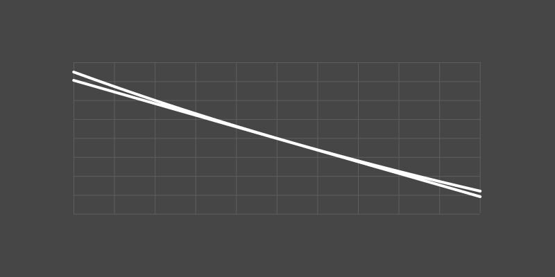
This is a difficult equation to work with. If we knew the moments of \(r_t\) I’m not sure how you would calculate the moments of \(R(r_t)\). However, this function appears to be almost linear. The chart below shows that this function is close to a straight line:
Notice that the ETF return is nearly a straight line. A slight bend in the line suggests that a second order Taylor expansion could be used to simplify \(R(r_t)\) and allow us to estimate the moments of \(R(r_t)\).
First order Taylor expansion
The first derivative is: $$ \begin{aligned} R^\prime(r_t) &=\frac{d}{dr_t} \frac{r_{t-1}}{r_t} - \frac{d}{dr_t} \left[\frac{r_{t-1}}{r_t} (1 + \frac{r_t}{p})^{-pT} \right] + \frac{d}{dr_t}(1 + \frac{r_t}{p})^{-pT} \\ &=\frac{d}{dr_t} \frac{r_{t-1}}{r_t} - \frac{d}{dr_t} \left[\frac{r_{t-1}}{r_t}\right] (1 + \frac{r_t}{p})^{-pT} - \frac{r_{t-1}}{r_t} \frac{d}{dr_t}\left[ (1 + \frac{r_t}{p})^{-pT}\right] + \frac{d}{dr_t}(1 + \frac{r_t}{p})^{-pT} \\ &=\frac{d}{dr_t} \left[\frac{r_{t-1}}{r_t}\right] \left(1 - (1 + \frac{r_t}{p})^{-pT}\right) + (1 - \frac{r_{t-1}}{r_t}) \frac{d}{dr_t}\left[ (1 + \frac{r_t}{p})^{-pT}\right] \\ \end{aligned} $$
We have: $$ \begin{equation} \frac{d}{dr_t} \frac{r_{t-1}}{r_t} = -\frac{r_{t-1}}{r_t^2} \label{1}\tag{1} \end{equation} $$ and (lazily) using Wolfram Alpha I get: $$ \begin{equation} \frac{d}{dr_t}(1 + \frac{r_t}{p})^{-pT} = -\frac{pT}{p + r_t} (\frac{p + r_t}{p})^{-pT} \label{2}\tag{2} \end{equation} $$ giving: $$ \begin{aligned} R^\prime(r_t) &= -\frac{r_{t-1}}{r_t^2} \left(1 - (1 + \frac{r_t}{p})^{-pT}\right) - (1 - \frac{r_{t-1}}{r_t})\frac{pT}{p + r_t} (\frac{p + r_t}{p})^{-pT} \\ \end{aligned} $$
The first order Taylor expansion is: $$ R_1(r_t) = R(r_{t-1}) + \frac{R^\prime(r_{t-1})}{1!}(r_t - r_{t-1}) $$
Because we have taken the Taylor expansion around \(r_{t-1}\) instead of 0, some of the terms in \(R(r_{t-1})\) and \(R^\prime(r_{t-1})\) cancel out giving: $$ \begin{aligned} R(r_{t-1}) &= \frac{r_{t-1}}{f} \\ R^\prime(r_{t-1}) &= -\frac{1}{r_{t-1}} \left(1 - (1 + \frac{r_{t-1}}{p})^{-pT}\right) \\ R_1(r_t) &= R(r_{t-1}) + R^\prime(r_{t-1})(r_t - r_{t-1}) \end{aligned} $$
You can see in the chart below that the first order expansion is a pretty good approximation. However, there does appear to be a bit of a curve to the function. A second order expansion would probably work better.
Second order Taylor expansion
Taking the second derivative is quite tedious. Starting off: $$ \begin{aligned} R^{\prime\prime}(r_t) = \frac{d}{dr_t}R^\prime(r_t) =& -\frac{d}{dr_t} \left[\frac{r_{t-1}}{r_t^2} \left(1 - (1 + \frac{r_t}{p})^{-pT}\right)\right] \\ & - \frac{d}{dr_t} \left[(1 - \frac{r_{t-1}}{r_t})\frac{pT}{p + r_t} (\frac{p + r_t}{p})^{-pT}\right] \\ \\ =& -\frac{d}{dr_t} \left[\frac{r_{t-1}}{r_t^2}\right] \left(1 - (1 + \frac{r_t}{p})^{-pT}\right) \\ & -\frac{r_{t-1}}{r_t^2} \frac{d}{dr_t} \left[\left(1 - (1 + \frac{r_t}{p})^{-pT}\right)\right] \\ & - \frac{d}{dr_t} \left[(1 - \frac{r_{t-1}}{r_t})\right]\frac{pT}{p + r_t} (\frac{p + r_t}{p})^{-pT} \\ & - (1 - \frac{r_{t-1}}{r_t})\frac{d}{dr_t}\left[\frac{pT}{p + r_t} (\frac{p + r_t}{p})^{-pT}\right] \\ \\ \end{aligned} $$ We have: $$ \frac{d}{dr_t} \frac{r_{t-1}}{r_t^2} = -2\frac{r_{t-1}}{r_t^3} $$ and using equations \(\eqref{1}\) & \(\eqref{2}\) we can solve the first three terms: $$ \begin{aligned} R^{\prime\prime}(r_t) =& \ 2\frac{r_{t-1}}{r_t^3} \left(1 - (1 + \frac{r_t}{p})^{-pT}\right) \\ & -\frac{r_{t-1}}{r_t^2}\frac{pT}{p + r_t} (\frac{p + r_t}{p})^{-pT} \\ & -\frac{r_{t-1}}{r_t^2}\frac{pT}{p + r_t} (\frac{p + r_t}{p})^{-pT} \\ & - (1 - \frac{r_{t-1}}{r_t})\frac{d}{dr_t}\left[\frac{pT}{p + r_t} (\frac{p + r_t}{p})^{-pT}\right] \\ \end{aligned} $$ The last term we will ignore because we are only interested in taking the second derivative at \(R^{\prime\prime}(r_{t-1})\) where the last term equals 0: $$ R^{\prime\prime}(r_{t-1}) = 2\frac{1}{r_{t-1}^2} \left(1 - (1 + \frac{r_{t-1}}{p})^{-pT}\right) -2\frac{1}{r_{t-1}}\frac{pT}{p + r_{t-1}} (\frac{p + r_{t-1}}{p})^{-pT} $$ Which gives us the second order Taylor expansion: $$ R_2(r_t) = R(r_{t-1}) + R^\prime(r_{t-1})(r_t - r_{t-1}) + R^{\prime\prime}(r_{t-1}) \frac{1}{2}(r_t - r_{t-1})^2 $$ We can rewrite this into a polynomial of \(r_t\) giving us a second order Taylor approximation to the original function: $$ \begin{aligned} R(r_{t-1}) &= \frac{r_{t-1}}{f} \\ R^\prime(r_{t-1}) &= -\frac{1}{r_{t-1}} \left(1 - (1 + \frac{r_{t-1}}{p})^{-pT}\right) \\ R^{\prime\prime}(r_{t-1}) &= 2\frac{1}{r_{t-1}^2} \left(1 - (1 + \frac{r_{t-1}}{p})^{-pT}\right) -2\frac{1}{r_{t-1}}\frac{pT}{p + r_{t-1}} (\frac{p + r_{t-1}}{p})^{-pT} \\ C_0 &= R(r_{t-1}) - R^\prime(r_{t-1})r_{t-1} + R^{\prime\prime}(r_{t-1}) \frac{1}{2}r_{t-1}^2 \\ C_1 &= R^\prime(r_{t-1}) - R^{\prime\prime}(r_{t-1}) r_{t-1} \\ C_2 &= R^{\prime\prime}(r_{t-1}) \frac{1}{2} \\ R_2(r_t) &= C_0 + C_1 r_t + C_2 r_t^2 \end{aligned} $$
This second order expansion fits much better than the first order. You can see in the chart below we are now correctly modelling the curve.
Moments of bond returns
In the previous section we derived the second order Taylor expansion of bond returns \(R_2(r_t)\). Here, we’ll derive the mean and variance of \(R_2(r_t)\) as functions of the moments of the yield \(r_t\).
The mean is an easy one: $$ \text{mean}[R_2(r_t)] = E[R_2(r_t)] = C_0 + C_1 E[r_t] + C_2 E[r_t^2] $$
From the definition of variance, we get: $$ \text{var}[R_2(r_t)] = E[(R_2(r_t) - E[R_2(r_t)])^2] = E[R_2(r_t)^2] - E[R_2(r_t)]^2 $$ where: $$ \begin{aligned} E[R_2(r_t)^2] &= E[(C_0 + C_1 r_t + C_2 r_t^2)(C_0 + C_1 r_t + C_2 r_t^2)] \\ &= E[C_0^2 + 2C_0C_1r_t + (2C_0 C_2 + C_1^2 )r_t^2 + 2C_1C_2 r_t^3 + C_2^2 r_t^4] \\ &= C_0^2 + 2C_0C_1E[r_t] + (2C_0 C_2 + C_1^2 )E[r_t^2] + 2C_1C_2 E[r_t^3] + C_2^2 E[r_t^4] \\ \end{aligned} $$
The mean and variance above require we know the first 4 raw moments of the yield: \(E[r_t]\), \(E[r_t^2]\), \(E[r_t^3]\) and \(E[r_t^4]\). Common models of interest rates assume a Gaussian distribution (for example Vasicek model) or a Log–normal distribution (for example Black–Karasinski model).
The table gives the Gaussian moments :
| Moment | Gaussian |
|---|---|
| \(E[r_t]\) | \(\mu\) |
| \(E[r_t^2]\) | \(\mu^2 + \sigma^2\) |
| \(E[r_t^3]\) | \(\mu^3 + 3\mu\sigma^2\) |
| \(E[r_t^4]\) | \(\mu^4 +6\mu^2\sigma^2 + 3\sigma^4\) |
The \(k^\text{th}\) Log–normal moment evaluates as 1 2: $$ E[r_t^k] = e^{\frac{k (2 \mu + k \sigma^2)}{2}} $$