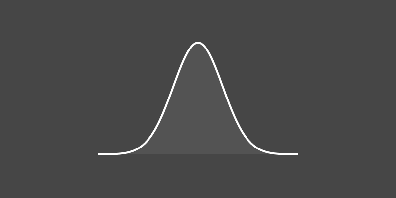
The moments of a statistical distribution are a family of quantities that describe the distribution’s shape. Moments include the familiar quantities mean, variance, skewness and kurtosis.
Moments are broken down into raw, central and standardised moments. They are also ordered. For example, variance is the second central moment. The first 4 sets of moments are:
| Order | Raw moments | Central moments | Standardised moments |
|---|---|---|---|
| 1 | \(E[X] = \mu\) | \(E[X - \mu] = 0\) | \(E[\frac{X - \mu}{\sigma}] = 0\) |
| 2 | \(E[X^2]\) | \(E[(X - \mu)^2] = \sigma^2\) | \(E[(\frac{X - \mu}{\sigma})^2] = 1\) |
| 3 | \(E[X^3]\) | \(E[(X - \mu)^3]\) | \(E[(\frac{X - \mu}{\sigma})^3] = s\) |
| 4 | \(E[X^4]\) | \(E[(X - \mu)^4]\) | \(E[(\frac{X - \mu}{\sigma})^4] = \kappa\) |
where \(\mu\) is the mean, \(\sigma^2\) is the variance, \(s\) is the skewness, and \(\kappa\) is the kurtosis.
Often, you can calculate the moments of a function of a random value based on the moments of that random variable. I frequently find myself calculating the moments of functions of Gaussian random variables. Here, I list out the moments of the Gaussian distribution for reference and describe a method for calculating co-moments.
Gaussian moments
If X is a Gaussian distribution, \(X \sim \mathcal{N}(\mu, \sigma^2)\), then the moments are 1 2:
| Raw moments | Central moments | Standardised moments |
|---|---|---|
| \(E[X] = \mu\) | \(E[X - \mu] = 0\) | \(E[\frac{X - \mu}{\sigma}] = 0\) |
| \(E[X^2] = \mu^2 + \sigma^2\) | \(E[(X - \mu)^2] = \sigma^2\) | \(E[(\frac{X - \mu}{\sigma})^2] = 1\) |
| \(E[X^3] = \mu^3 + 3\mu\sigma^2\) | \(E[(X - \mu)^3] = 0\) | \(E[(\frac{X - \mu}{\sigma})^3] = 0 = s\) |
| \(E[X^4] = \mu^4 +6\mu^2\sigma^2 + 3\sigma^4\) | \(E[(X - \mu)^4] = 3\sigma^4\) | \(E[(\frac{X - \mu}{\sigma})^4] = 3 = \kappa\) |
Gaussian co-moments
Co-moments involve multiple random variables. For example, \(E[XY]\) is a co-moment of \(X\) and \(Y\). These can be fairly tedious to derive and require a trick.
How to derive
The trick to deriving Gaussian co-moments is to write the two variables as linear combinations of three standard normal distributions (\(\hat{X},\hat{Y},\hat{Z} \sim \mathcal{N}(0, 1)\)). Then, expand out the expected value into combinations of \(E[\hat{X}^i\hat{Y}^j\hat{Z}^k]\) which resolve to \(E[\hat{X}^i]E[\hat{Y}^j]E[\hat{Z}^k]\) 3.
Say we have two Gaussian random variables \(X\) and \(Y\) with means \(\mu_X\) and \(\mu_Y\), variances \(\sigma^2_X\) and \(\sigma^2_Y\) and covariance \(\sigma^2_{XY}\). We can write these two variables as functions of three uncorrelated standard normals \(\hat{X}\), \(\hat{Y}\) and \(\hat{Z}\): $$ \begin{aligned} \hat{\sigma}_X &= \sqrt{\sigma^2_X - \sigma^2_{XY}} \\ \hat{\sigma}_Y &= \sqrt{\sigma^2_Y - \sigma^2_{XY}} \\ \\ X &= \mu_X + \hat{\sigma}_X \hat{X} + \sigma_{XY} \hat{Z} \\ Y &= \mu_Y + \hat{\sigma}_Y \hat{Y} + \sigma_{XY} \hat{Z} \\ \end{aligned} $$
We can check these formulas by checking that the variance and covariance resolve to \(\sigma^2_X\), \(\sigma^2_Y\) and \(\sigma^2_{XY}\). The variance of summed independent Gaussians is the sum of the variances, and so: $$ \text{var}[X] = \hat{\sigma}_X^2 + \sigma_{XY}^2= \sigma^2_X $$ \(Y\) resolves the same. And the covariance: $$ \begin{aligned} \text{cov}[X,Y] &= E[(\hat{\sigma}_X \hat{X} + \sigma_{XY} \hat{Z})(\hat{\sigma}_Y \hat{Y} + \sigma_{XY} \hat{Z})] \\ &= E[\hat{\sigma}_X \hat{\sigma}_Y \hat{X} \hat{Y} + \hat{\sigma}_X \sigma_{XY} \hat{X} \hat{Z} + \sigma_{XY}\hat{\sigma}_Y \hat{Y} \hat{Z} + \sigma_{XY}^2 \hat{Z}^2] \\ &= \hat{\sigma}_X \hat{\sigma}_Y E[\hat{X} \hat{Y}] + \hat{\sigma}_X \sigma_{XY} E[\hat{X} \hat{Z}] + \sigma_{XY}\hat{\sigma}_Y E[\hat{Y} \hat{Z}] + \sigma_{XY}^2 E[\hat{Z}^2] \\ &= \sigma_{XY}^2 \\ \end{aligned} $$
Derivations
We can use this method of rewriting into a combination of 3 standard normals to derive various co-moments. First expand out the two Gaussians: $$ \begin{aligned} E[XY] &= E[(\mu_X + \hat{\sigma}_X \hat{X} + \sigma_{XY} \hat{Z})(\mu_Y + \hat{\sigma}_Y \hat{Y} + \sigma_{XY} \hat{Z})] \\ &= \mu_X\mu_Y + \mu_X\hat{\sigma}_Y E[\hat{Y}] + \mu_X\sigma_{XY} E[\hat{Z}]\\ &\quad + \hat{\sigma}_X\mu_Y E[\hat{X}] + \hat{\sigma}_X \hat{\sigma}_Y E[\hat{X}\hat{Y}] + \hat{\sigma}_X \sigma_{XY} E[\hat{X}\hat{Z}]\\ &\quad + \sigma_{XY}\mu_Y E[\hat{Z}] + \sigma_{XY} \hat{\sigma}_Y E[\hat{Y}\hat{Z}] + \sigma_{XY}^2 E[\hat{Z}^2]\\ \end{aligned} $$ Then, expand the monomials from \(E[\hat{X}^i\hat{Y}^j\hat{Z}^k]\) to \(E[\hat{X}^i]E[\hat{Y}^j]E[\hat{Z}^k]\): $$ \begin{aligned} &= \mu_X\mu_Y + \mu_X\hat{\sigma}_Y E[\hat{Y}] + \mu_X\sigma_{XY} E[\hat{Z}]\\ &\quad + \hat{\sigma}_X\mu_Y E[\hat{X}] + \hat{\sigma}_X \hat{\sigma}_Y E[\hat{X}]E[\hat{Y}] + \hat{\sigma}_X \sigma_{XY} E[\hat{X}]E[\hat{Z}]\\ &\quad + \sigma_{XY}\mu_Y E[\hat{Z}] + \sigma_{XY} \hat{\sigma}_Y E[\hat{Y}]E[\hat{Z}] + \sigma_{XY}^2 E[\hat{Z}^2]\\ \end{aligned} $$ And replace all the Gaussian moments with their values from the table above (for example \(E[\hat{Y}] = 0\)): $$ E[XY] = \mu_X\mu_Y + \sigma_{XY}^2 \tag{1} $$
Two other co-moments that come up often are: $$ \begin{aligned} E[X^2Y] &= E[(\mu_X + \hat{\sigma}_X \hat{X} + \sigma_{XY} \hat{Z})^2(\mu_Y + \hat{\sigma}_Y \hat{Y} + \sigma_{XY} \hat{Z})] \\ &= \mu_X^2\mu_Y + 2 \mu_X\sigma_{XY}^2 + \mu_Y\sigma^2_X \label{2}\tag{2} \end{aligned} $$
$$ \begin{aligned} E[X^2Y^2] &= E[(\mu_X + \hat{\sigma}_X \hat{X} + \sigma_{XY} \hat{Z})^2(\mu_Y + \hat{\sigma}_Y \hat{Y} + \sigma_{XY} \hat{Z})^2] \\ &= \sigma^2_X\sigma^2_Y + \sigma^2_X \mu_{Y}^{2} + \sigma^2_Y \mu_{X}^{2} + 2 \sigma_{XY}^{4} + 4 \mu_{X} \mu_{Y} \sigma_{XY}^{2} + \mu_{X}^{2} \mu_{Y}^{2} \label{3}\tag{3} \end{aligned} $$


