I’ve come across trading systems that spew out 10s of gigabytes of logs per day. When something goes wrong, some poor intern would have to grep through these log files to figure out why it broke – sometimes for days.

The thing is, logs should not be human readable. These days, computer systems generate so many logs that we need tools to parse and understand them. Human’s no longer read logs, machines do.

When coming across trading systems spewing out gigabytes of logs, I bank a quick win by converting these logs into JSON. I can then stream these logs into a time series database and visualise them with my favourite dashboard. That way, I can see exactly what is going on in near real time and catch problems early.

Here, we’re going to create a trading app demo that logs to JSON and a system that ships these logs into a time series database and visualises them.

The steps involved are:

1. Create an app that logs a price
2. Switch to JSON logs
3. Setup time series database
4. Setup a log shipper to move logs into the time series database
5. Visualise the data

You can find all the code here in a Github repository monitoring-trading-systems.

1. Create an app

For our trading app, we’ll use a script that logs a random price:

# filename: trader.py
from time import sleep
import numpy as np
import logging
import os

LOG_FILE_NAME = os.environ['LOG_FILE_NAME']

logger = logging.getLogger()
logger.setLevel(logging.DEBUG)
console_handler = logging.StreamHandler()
logger.addHandler(console_handler)
file_handler = logging.FileHandler(LOG_FILE_NAME)
logger.addHandler(file_handler)

price = 100

while True:
    price = price * (1 + np.random.randn() * 0.01)
    logger.info(f"price {price}")
    sleep(0.5)

This app sets up a logger that prints to the console and dumps to a log file LOG_FILE_NAME. The logs look like:

price 101.50747597319688
price 101.45122289615952
price 102.82811428242694

Dockerising the app

Dockerising the trading app makes integrating with the monitoring services easier later. Setup your file structure like this:

repo/
├── trader/
│   ├── Dockerfile
│   └── trader.py
└── docker-compose.yml

In the Dockerfile we want to setup a simple python environment with the two required packages numpy and structlog:

# filename: Dockerfile
FROM python:3.11.0-slim-buster

RUN pip install numpy==1.23.5 structlog==22.3.0

WORKDIR /app
COPY trader.py /app/trader.py

We want to be able to run this app with the command docker-compose up so put the following into the docker-compose.yml file:

# filename: docker-compose.yml
version: '3.7'

services:
  trader:
    build:
      context: ./trader
    container_name: trader
    command: python trader.py
    environment:
      - LOG_FILE_NAME=/var/log/trader/trader.logs
    volumes:
      - logdata:/var/log/trader

volumes:
  logdata:

Here we’ve told Docker to build the service called trader which runs the command python trader.py in the container and stores the logs in a volume called logdata.

If you go ahead and run the following command you will see logs in your console:

docker-compose up

2. Switch to JSON logs

The Python package structlog creates structured logs for you. The package includes a JSON formatter which we’re going to use.

Setting up JSON logs is as easy as configuring structlog and wrapping the default logger from our demo trading app above. The updated trader.py script looks like:

from time import sleep
import numpy as np
import structlog
import logging
import os

LOG_FILE_NAME = os.environ['LOG_FILE_NAME']

logger = logging.getLogger()
logger.setLevel(logging.DEBUG)
console_handler = logging.StreamHandler()
logger.addHandler(console_handler)
file_handler = logging.FileHandler(LOG_FILE_NAME)
logger.addHandler(file_handler)

# Configure the structured logger
structlog.configure_once(
    processors=[
        structlog.stdlib.add_log_level,
        structlog.processors.TimeStamper(fmt="iso", utc=True),
        structlog.processors.JSONRenderer(),
    ],
)

# Wrap the root logger with the structured logger
json_logger = structlog.wrap_logger(logger)

price = 100

while True:
    price = price * (1 + np.random.randn() * 0.01)

    # Log price in JSON
    json_logger.info(event="price_log", price=price)

    sleep(0.5)

A log is a statement that something happened. In other words, an event. structlog has the required argument event="NAME". Best practice is for each of your logs to have their own event name. That way, you can always pick out the exact logs you want down stream.

Now, the trading app’s logs look like:

{"price": 98.29655117355337, "event": "price", "level": "info", "timestamp": "2022-12-14T06:21:05.874105Z"}
{"price": 99.25440619746382, "event": "price", "level": "info", "timestamp": "2022-12-14T06:21:06.375861Z"}
{"price": 100.36139973205326, "event": "price", "level": "info", "timestamp": "2022-12-14T06:21:06.877588Z"}
{"price": 98.746303446643, "event": "price", "level": "info", "timestamp": "2022-12-14T06:21:07.380507Z"}

Perfectly machine readable.

3. Setup time series database

We’re going to use QuestDB as our time series database. QuestDB ingests logs lightening fast and returns SQL queries in milliseconds.

QuestDB is free and open source. You can add a QuestDB service to the docker-compose.yml file with:

questdb:
  image: questdb/questdb:7.1.1
  container_name: questdb
  ports:
    - "9000:9000"  # Rest and Web app
    - "9009:9009"  # InfluxDB line protocol
    - "8812:8812"  # Postgres protocol
  healthcheck:
    test: timeout 10s bash -c ':> /dev/tcp/localhost/9003'
    interval: 5s
    timeout: 10s
    retries: 50

Here, we’ve instructed Docker to leave open three ports:

• 9000 gives you a web app to play with QuestDB
• 9009 is the port we will send logs to
• 8812 is the port we’ll use to run SQL queries

Take note of the health check. QuestDB can take a moment to start up. We will want services that depend on it to wait before trying to connect. By adding the health check, Docker will know to wait until QuestDB is ready.

4. Setup a log shipper

We need a way of moving logs from the trader.logs file into QuestDB. Programs that move logs are often termed log shippers.

In this setup, we’ll be using Telegraf.

Telegraf is ideal because it is able to read JSON logs and send them in InfluxDB’s Line Protocol format via TCP. QuestDB accepts logs in InfluxDB’s Line Protocol format on port 9009.

Telegraf uses a telegraf.conf file for configuration. We want to tell Filebeat where the log file lives and where QuestDB lives. We can do this with:

# filename: telegraf.conf
[agent]
  # Default data collection interval for all inputs
  interval = "1s"

  # Default flushing interval for all outputs
  flush_interval = "1s"

[[inputs.tail]]
  files = ["$LOG_FILE_NAME"]
  from_beginning = true

  json_string_fields = [
    "level",
  ]

  data_format = "json"
  json_strict = true
  json_name_key = "event"
  json_time_key = "timestamp"
  json_time_format  = "2006-01-02T15:04:05.999999Z"

[[outputs.socket_writer]]
  address = "tcp://$QUESTDB_HOST_NAME"
  data_format = "influx"

The Telegraf service can then be created with:

telegraf:
  image: telegraf:1.26.2
  container_name: telegraf
  environment:
    - QUESTDB_HOST_NAME=questdb:9009
    - LOG_FILE_NAME=/var/log/trader/trader.logs
  depends_on:
    questdb:
      condition: service_healthy
  volumes:
    - logdata:/var/log/trader
    - ./telegraf.conf:/etc/telegraf/telegraf.conf

Here we’ve told Docker to give telegraf access to the same volume (logdata) as the trader service. This means that telegraf can read the logs produced by trader.

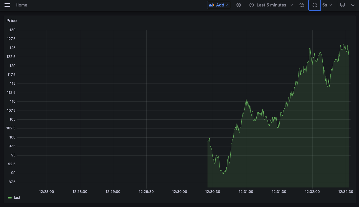
5. Visualise

We’ve now got a trading app dumping JSON logs to a file and these logs are being streamed into a database. All we have left to do is visualise the data.

Grafana is an open source visualisation tool that excels at metrics and time series.

Add Grafana as a service to your docker-compose.yml file:

  grafana:
    image: grafana/grafana:9.5.1
    ports:
      - "3000:3000"
    environment:
      - QUESTDB_URL=questdb:8812
      - GF_SECURITY_ADMIN_USER=admin
      - GF_SECURITY_ADMIN_PASSWORD=admin
      - GF_AUTH_BASIC_ENABLED=false
      - GF_AUTH_ANONYMOUS_ENABLED=true
      - GF_AUTH_ANONYMOUS_ORG_ROLE=Editor
    depends_on:
      questdb:
        condition: service_healthy

When running, you can navigate to localhost:3000 to explore Grafana.

Configuration

Grafana’s UI allows you to connect to QuestDB and begin exploring.

A fantastic feature of Grafana is defining all configuration in code. This includes the database connection and dashboards. That’s all a little involved to walk through here. However, the accompanying Github repository is setup with a Grafana service configured to talk to QuestDB, and has a ready built dashboard for you to explore.

Accompanying Repository

To see this whole monitoring system in action, clone the repository and spin up the stack:

git clone https://github.com/robolyst/trading-monitoring-demo
cd trading-monitoring-demo
docker-compose up

You’ll get a spew of logs on the screen. Wait a moment and then open the dashboard at http://localhost:3000/

Footnotes

Corrections

If you see any mistakes or room for improvement, please reach out to me on Twitter @DrAdrian.

Citation

Please cite this work as:

Letchford (2023), "How to engineer a monitoring system for your trading strategy", OS Quant.

In BibTeX please use:

@article{Letchford2023,
    author = {Letchford, Adrian},
    title = {How to engineer a monitoring system for your trading strategy},
    journal = {OS Quant},
    year = {2023},
    note = {https://osquant.com/papers/monitoring-trading-systems/},
}