For decades, researchers have noted properties of returns that are consistent across different assets. These properties have become known as stylized facts. They are measurable, but, researchers have not been able to prove that they must be true.
The common stylized facts we are interested in here are 1:
- Returns are not Gaussian.
- Returns have fat tails.
- Returns become more Gaussian on higher time frames and less Gaussian on lower time frames.
I want to show you why these three properties actually make sense, even if we cannot prove that they are true. I’ll explain the first property based on the definition of a Gaussian distribution. The second and third can be shown if some intuitive assumptions are made.
I’ll start by breaking down the Gaussian distribution.
What is a Gaussian distribution?
The probability density function of a Gaussian distribution is depicted in the figure below and described by the following equation:
$$ f(x) = \frac{1}{\sigma\sqrt{2\pi}}e^{-\frac{1}{2}(\frac{x-\mu}{\sigma})^2} $$
The Gaussian distribution turns up everywhere, and with good reason. It describes the average of \(n\) independently and identically distributed random samples from any distribution as \(n\) tends to infinity:
$$ \frac{X_1 + \dots + X_n}{n} \sim \mathcal{N}(\mu, \sigma^2) $$
We know this is true from the central limit theorem.
We can actually make the Gaussian distribution a bit more general. A Gaussian variable multiplied by some constant is still Gaussian. This means we can multiply an average value by the number of samples to turn it into a sum:
$$ X_1 + \dots + X_n \sim n\mathcal{N}(\mu, \sigma^2) = \mathcal{N}(n\mu, n\sigma^2) $$
A Gaussian distribution models the sum of \(n\) independently and identically distributed random values as \(n\) tends to infinity.
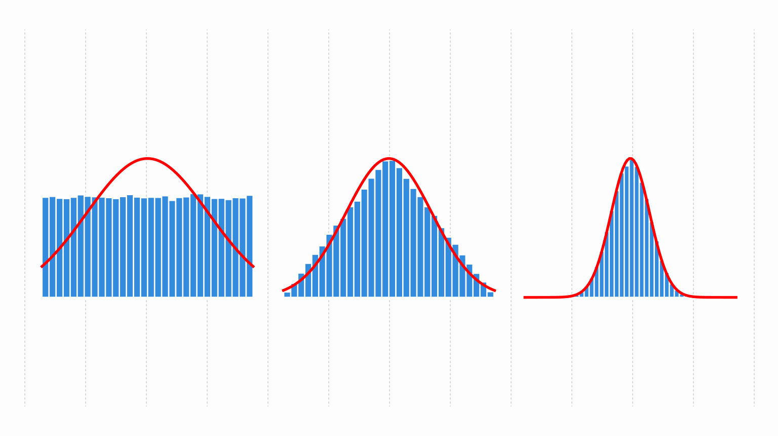
We can see this in action by taking \(n\) samples from a uniform distribution, summing, and plotting the distribution of those sums:

Returns are not Gaussian
The first stylized fact is that returns are not Gaussian. It turns out, returns do not meet the assumptions of a Gaussian distribution.
For this discussion, we are going to think in terms of logged prices. That is, when I say “return” I mean change in logged price:
$$ \text{return at time } t = \frac{p_t - p_{t-1}}{p_{t-1}} \approx \log(p_t) - \log(p_{t-1}) $$
This means we can think of returns as summing together rather than multiplying together.
A daily return is the sum of a fixed number of returns. As an example, we’ll say that a day is made up of 8 trading hours. Since we know that a sum of \(n = 8\) values is approximately Gaussian, it makes sense that the daily returns ought to be Gaussian. To see why this isn’t the case, we need to break down a day’s return to its atomic level. Each hourly return is the sum of minutely returns which are the sum of per second returns. If we continue this logic, we get to the atomic level: ticks.
Each day’s return is a sum of tick returns. The key thing to note is that each day has a different number of ticks. Bringing this back to the Gaussian distribution, each day is the sum of a different number of ticks. The \(n\) is different on each day. The Gaussian distribution assumes that \(n\) is the same for each sample. Therefore, returns on any time scale do not meet the assumptions of a Gaussian distribution.
Returns have fat tails
We need to make two assumptions to show that fat tails make sense. First that ticks, $T$, are drawn from a Gaussian distribution. Second that returns, $R$, are a sum of $N$ ticks where $N$ is drawn from a Poisson distribution. This is written as: $$ \begin{aligned} T &\sim \mathcal{N}(\mu, \sigma^2) \\ N &\sim \text{Poisson}(\lambda) \\ R &\sim \mathcal{N}(N\mu, N\sigma^2) \\ \end{aligned} $$
This is a type of compound Poisson distribution.
By making ticks Gaussian, we guarantee that their sum is also Gaussian. Which means that any deviation from a Gaussian distribution will have to come from summing together $N \sim \text{Poisson}$ values.
A distribution’s tails are measured with the fourth standard moment commonly known as kurtosis. A Gaussian distribution has a kurtosis of 3. If a distribution has a kurtosis larger than 3, then it has fatter tails than a Gaussian distribution. Therefore, we need to show that $\text{kurtosis}(R) > 3$.
Using the method of moments in the appendix we show that: $$ \text{kurtosis}(R) = 3 + \frac{E[T^4]}{\lambda E[T^2]^2} $$
Both $E[T^4]$ and $E[T^2]$ are positive values. Therefore, $\text{kurtosis}(R) > 3$ which means that a Poisson sum of ticks is not Gaussian and has fatter tails.
More Gaussian at higher time frames
The last stylized fact I want to touch on is the observation that returns become more Gaussian on higher time frames. That is, weekly returns look more Gaussian than hourly returns.
Higher time frames mean that returns are sums of more ticks, or, larger $N$ in the compound Poisson model we’re using. Getting larger values for $N$ means the expected value $E[N] = \lambda$ is larger. This is equivalent to larger values for $\lambda$.
As $\lambda$ gets bigger and bigger, $\text{kurtosis}(R)$ asymptotes towards 3: $$ \lim_{\lambda \to \infty} \text{kurtosis}(R) = \lim_{\lambda \to \infty} \left[ 3 + \frac{E[T^4]}{\lambda E[T^2]^2} \right]= 3 $$
A kurtosis of $3$ is the same as a Gaussian distribution. This means, under the compound Poisson model, as the expected number of ticks increases returns become more Gaussian.
Conclusions
Three of the common stylized facts about returns appear to make sense:
- Returns are not Gaussian makes sense because a Gaussian distribution models the sum of \(n\) things but returns are the sum of varying amounts of ticks.
- Returns have fat tails makes sense because we get fat tails when each sample is the sum of a different number of things.
- More Gaussian at higher time frames makes sense because when each sample is the sum of a different number of things, kurtosis asymptotes to 3 as the number of things increases to infinity. A Gaussian distribution has a kurtosis of 3.
These are not the only explanations for returns not being Gaussian. For example, overnight shocks can cause the opening price to be wildly different from the previous day’s close. The model in this paper does not include such shocks.
Appendix
Deriving kurtosis
There’s a paper which shows the statistics of a compound Poisson distribution2. However, I’m not sure how they derived the values. Here, I will use the method of moments to derive the kurtosis of a Poisson sum of Gaussians. The derivation just uses algebra, though it is a little tedious.
The kurtosis of $R$ is:
$$ \text{kurtosis}(R) = E\left[\left(\frac{R - \mu_R}{\sigma}\right)^4\right] = \frac{E[(R - \mu_R)^4]}{E[(R - \mu_R)^2]^2} $$
The value $E[(R - \mu_R)^4]$ is known as the fourth central moment and $E[(R - \mu_R)^2]$ is the second central moment or variance. Both of these can be expanded into raw moments:
$$ \begin{aligned} E[(R - \mu_R)^2] &= E[R^2] - E[R]^2 \\ E[(R - \mu_R)^4] &= E[R^4] - 4 E[R]E[R^3] + 6 E[R]^2E[R^2] - 3E[R]^4 \\ \end{aligned} $$
Each of the raw moments of $R$ can be written as functions of the raw moments of $T$ and $N$. To do this, we need a table of the raw moments of a Gaussian distribution ($T$)3 and a Poisson distribution ($N$) 4 5:
| Gaussian raw moments | |
|---|---|
| 1 | $E[T] = \mu$ |
| 2 | $E[T^2] = \mu^2 + \sigma^2$ |
| 3 | $E[T^3] = \mu^3 + 3\mu\sigma^2$ |
| 4 | $E[T^4] = \mu^4 +6\mu^2\sigma^2 + 3\sigma^4$ |
| Poisson raw moments | |
|---|---|
| 1 | $E[N] = \lambda$ |
| 2 | $E[N^2] = \lambda^2 + \lambda$ |
| 3 | $E[N^3] = \lambda^3 + 3\lambda^2 + \lambda$ |
| 4 | $E[N^4] = \lambda^4 + 6\lambda^3 + 7\lambda^2 + \lambda$ |
We note that $E[R^n]$ can be expanded with6: $$ E[R^n] = E[E[R^n|N]] $$ Where $E[R^n|N]$ is a raw moment of a Gaussian distribution. Expanding the first raw moment we get: $$ E[R] = E[E[R|N]] = E[N]\mu = \lambda\mu $$ The second raw moment: $$ \begin{aligned} E[R^2] &= E[E[R^2|N]] \\ &= E[N^2]\mu^2 + E[N]\sigma^2 \\ &= (\lambda^2 + \lambda)\mu^2 + \lambda\sigma^2 \\ &= \lambda^2\mu^2 + \lambda(\mu^2 + \sigma^2) \\ &= \lambda^2\mu^2 + \lambda E[T^2] \\ \end{aligned} $$ The third raw moment: $$ \begin{aligned} E[R^3] &= E[E[R^3|N]] \\ &= E[N^3]\mu^3 + 3 E[N^2]\mu\sigma^2 \\ &= (\lambda^3 + 3\lambda^2 + \lambda)\mu^3 + 3 (\lambda^2 + \lambda)\mu\sigma^2 \\ &= \lambda^3\mu^3 + 3\lambda^2\mu^3 + \lambda\mu^3 + 3\lambda^2\mu\sigma^2 + 3\lambda\mu\sigma^2 \\ &= \lambda^3\mu^3 + 3\lambda^2\mu^3 + 3\lambda^2\mu\sigma^2 + \lambda E[T^3] \\ &= \lambda^3\mu^3 + 3\lambda^2\mu(\mu^2 + \sigma^2) + \lambda E[T^3] \\ &= \lambda^3\mu^3 + 3\lambda^2\mu E[T^2] + \lambda E[T^3] \\ \end{aligned} $$
The fourth raw moment: $$ \begin{aligned} E[R^4] &= E[E[R^4|N]] \\ &= E[N^4]\mu^4 +6E[N^3]\mu^2\sigma^2 + 3 E[N^2]\sigma^4 \\ &= (\lambda^4 + 6\lambda^3 + 7\lambda^2 + \lambda)\mu^4 +6(\lambda^3 + 3\lambda^2 + \lambda)\mu^2\sigma^2 + 3 (\lambda^2 + \lambda)\sigma^4 \\ &= \lambda^4\mu^4 + 6\lambda^3\mu^4 + 7\lambda^2\mu^4 + \lambda\mu^4 + 6\lambda^3\mu^2\sigma^2 + 18\lambda^2\mu^2\sigma^2 + 6\lambda\mu^2\sigma^2 + 3 \lambda^2\sigma^4 + 3\lambda\sigma^4 \\ &= \lambda^4\mu^4 + 6\lambda^3\mu^4 + 7\lambda^2\mu^4 + 6\lambda^3\mu^2\sigma^2 + 18\lambda^2\mu^2\sigma^2 + 3 \lambda^2\sigma^4 + \lambda\mu^4 + 6\lambda\mu^2\sigma^2 + 3\lambda\sigma^4 \\ &= \lambda^4\mu^4 + 6\lambda^3\mu^4 + 7\lambda^2\mu^4 + 6\lambda^3\mu^2\sigma^2 + 18\lambda^2\mu^2\sigma^2 + 3 \lambda^2\sigma^4 + \lambda(\mu^4 + 6\mu^2\sigma^2 + 3 \sigma^4) \\ &= \lambda^4\mu^4 + 6\lambda^3\mu^4 + 7\lambda^2\mu^4 + 6\lambda^3\mu^2\sigma^2 + 18\lambda^2\mu^2\sigma^2 + 3 \lambda^2\sigma^4 + \lambda E[T^4] \\ &= \lambda^4\mu^4 + 7\lambda^2\mu^4 + 6\lambda^3\mu^2 E[T^2] + 18\lambda^2\mu^2\sigma^2 + 3 \lambda^2\sigma^4 + \lambda E[T^4] \\ \end{aligned} $$
Putting these raw moments into the second central moment we get: $$ \begin{aligned} E[(R - \mu_R)^2] &= E[R^2] - E[R]^2 \\ &= \lambda^2\mu^2 + \lambda E[T^2] - \lambda^2\mu^2 \\ &= \lambda E[T^2] \\ \end{aligned} $$
Similarly, putting these raw moments into the fourth central moment, we get: $$ \begin{aligned} E[(R - \mu_R)^4] &= E[R^4] - 4 E[R]E[R^3] + 6 E[R]^2E[R^2] - 3E[R]^4 \\ &= E[R^4] - 4 \lambda\mu E[R^3] + 6 \lambda^2 \mu^2 E[R^2] - 3\lambda^4\mu^4 \\ \end{aligned} $$ Expanding out \(E[R^2]\): $$ \begin{aligned} &= E[R^4] - 4 \lambda\mu E[R^3] + 6 \lambda^2 \mu^2 (\lambda^2\mu^2 + \lambda E[T^2]) - 3\lambda^4\mu^4 \\ &= E[R^4] - 4 \lambda\mu E[R^3] + 6 (\lambda^4\mu^4 + \lambda^3 \mu^2 E[T^2]) - 3\lambda^4\mu^4 \\ &= E[R^4] - 4 \lambda\mu E[R^3] + 6 \lambda^4\mu^4 + 6\lambda^3 \mu^2 E[T^2] - 3\lambda^4\mu^4 \\ &= E[R^4] - 4 \lambda\mu E[R^3] + 3 \lambda^4\mu^4 + 6\lambda^3 \mu^2 E[T^2] \\ \end{aligned} $$ Expanding out \(E[R^3]\): $$ \begin{aligned} &= E[R^4] - 4 \lambda\mu (\lambda^3\mu^3 + 3\lambda^2\mu E[T^2] + \lambda E[T^3]) + 3 \lambda^4\mu^4 + 6\lambda^3 \mu^2 E[T^2] \\ &= E[R^4] - 4 (\lambda^4\mu^4 + 3\lambda^3\mu^2 E[T^2] + \lambda^2\mu E[T^3]) + 3 \lambda^4\mu^4 + 6\lambda^3 \mu^2 E[T^2] \\ &= E[R^4] - 4 \lambda^4\mu^4 - 12\lambda^3\mu^2 E[T^2] - 4\lambda^2\mu E[T^3] + 3 \lambda^4\mu^4 + 6\lambda^3 \mu^2 E[T^2] \\ &= E[R^4] - \lambda^4\mu^4 - 12\lambda^3\mu^2 E[T^2] - 4\lambda^2\mu E[T^3] + 6\lambda^3 \mu^2 E[T^2] \\ &= E[R^4] - \lambda^4\mu^4 - 6\lambda^3\mu^2 E[T^2] - 4\lambda^2\mu E[T^3] \\ &= E[R^4] - \lambda^4\mu^4 - 6\lambda^3\mu^2 E[T^2] - 4\lambda^2\mu E[T^3] \\ \end{aligned} $$ Expanding out \(E[R^4]\): $$ \begin{aligned} &= \lambda^4\mu^4 + 7\lambda^2\mu^4 + 6\lambda^3\mu^2 E[T^2] + 18\lambda^2\mu^2\sigma^2 + 3 \lambda^2\sigma^4 + \lambda E[T^4] \\ & \quad - \lambda^4\mu^4 - 6\lambda^3\mu^2 E[T^2] - 4\lambda^2\mu E[T^3] \\ &= 7\lambda^2\mu^4 + 6\lambda^3\mu^2 E[T^2] + 18\lambda^2\mu^2\sigma^2 + 3 \lambda^2\sigma^4 + \lambda E[T^4] \\ & \quad - 6\lambda^3\mu^2 E[T^2] - 4\lambda^2\mu E[T^3] \\ &= 7\lambda^2\mu^4 + 18\lambda^2\mu^2\sigma^2 + 3 \lambda^2\sigma^4 + \lambda E[T^4] - 4\lambda^2\mu E[T^3] \\ &= 7\lambda^2\mu^4 + 18\lambda^2\mu^2\sigma^2 + 3 \lambda^2\sigma^4 + \lambda E[T^4] - 4\lambda^2\mu (\mu^3 + 3\mu\sigma^2) \\ &= 7\lambda^2\mu^4 + 18\lambda^2\mu^2\sigma^2 + 3 \lambda^2\sigma^4 + \lambda E[T^4] - 4\lambda^2\mu^4 - 12\lambda^2\mu^2\sigma^2 \\ &= 7\lambda^2\mu^4 + 6\lambda^2\mu^2\sigma^2 + 3 \lambda^2\sigma^4 + \lambda E[T^4] - 4\lambda^2\mu^4 \\ &= 3\lambda^2\mu^4 + 6\lambda^2\mu^2\sigma^2 + 3 \lambda^2\sigma^4 + \lambda E[T^4] \\ E[(R - \mu_R)^4] &= 3\lambda^2 E[T^2]^2 + \lambda E[T^4] \\ \end{aligned} $$
And putting these central moments back into kurtosis: $$ \begin{aligned} \text{kurtosis}(R) &= \frac{E[(R - \mu_R)^4]}{E[(R - \mu_R)^2]^2} \\ &= \frac{3\lambda^2 E[T^2]^2 + \lambda E[T^4]}{\lambda^2 E[T^2]^2} \\ &= \frac{3\lambda^2 E[T^2]^2}{\lambda^2 E[T^2]^2} + \frac{\lambda E[T^4]}{\lambda^2 E[T^2]^2} \\ &= 3 + \frac{E[T^4]}{\lambda E[T^2]^2} \\ \end{aligned} $$
If we assume that $\mu = 0$ then: $$ \begin{aligned} \text{kurtosis}(R|\mu = 0) &= 3 + \frac{E[T^4]}{\lambda E[T^2]^2} \\ &= 3 + \frac{3 \sigma^4}{\lambda \sigma^4} \\ &= 3 + \frac{3}{\lambda} \\ \end{aligned} $$