The Wiener-Khinchin theorem provides a clever way of building Gaussian processes for regression. I’ll show you this theorem in action with some Python code and how to use it to model a process.
The Wiener-Khinchin theorem states that an autocovariance function of a weakly stationary process is a function of the power spectral density and vice versa. These two are called Fourier duals and can be written as1: $$ \begin{align} \kappa(h) &= \int S(\omega) e^{2 \pi i \omega h} d \omega \label{1}\tag{1} \\ S(\omega) &= \int \kappa(h) e^{-2 \pi i \omega h} d h \\ \end{align} $$ Where $\kappa(h)$ is an autocovariance function of a process at lag $h$ and $S(\omega)$ is the power spectral density of the same process at frequency $\omega$. They are Fourier transforms of each other—hence the term Fourier duals.
The idea here is that if you want to model a process, you could estimate its power spectrum ($S$), calculate the autocovariance function using equation ($\ref{1}$) and construct a Gaussian process.
The problem is that equation ($\ref{1}$) is in continuous time and we generally work with discretely sampled time series. Luckily, there is a method known as the periodogram which is a discrete estimate of the power spectral density. SciPy provides this estimate under scipy.signal.periodogram. Now, equation ($\ref{1}$) can be treated discretely as:
$$ \kappa(h) = \sum_{\omega} S(\omega) e^{2 \pi i \omega h} d \omega \label{2}\tag{2} $$
Let’s try this out with some Python code.
Estimating the autocovariance function
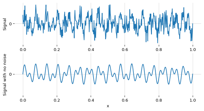
Generate a time series made up of two frequencies and some noise:
from numpy import sin, pi, cumsum, linspace
from numpy.random import seed, randn

seed(1)

N = 500  # Number of samples
x = linspace(0, 1, N)  # One interval
y = (
    sin(x * 2 * pi * 16)    # Oscillate 16 times per interval
    + sin(x * 2 * pi * 30)  # + 30 times per interval
    + randn(N)              # + some noise
)
Which looks like this:
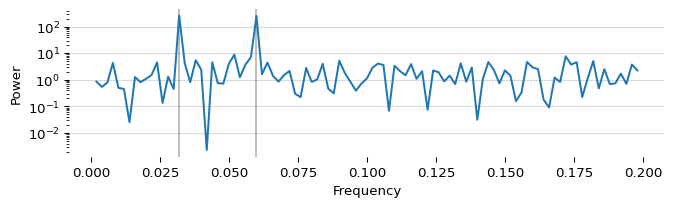
We can get the periodogram with:
from scipy.signal import periodogram
frequency, power = periodogram(y)
The array power is a noisy power spectrum with two spikes. One spike at $\frac{16}{N}$ and the other at $\frac{30}{N}$. It looks like:
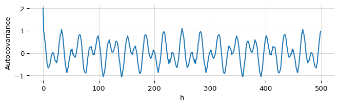
We can create a function that uses periodogram and equation ($\ref{2}$) to give us the autocovariance at each $h$ from $0$ to $N$:
import numpy as np
from scipy.signal import periodogram

def spectral_autocov(y):
    N = len(y)

    frequency, power = periodogram(y, nfft=N)
    d = np.mean(np.diff(frequency))

    autocov = np.real([
        np.sum(np.exp(2 * np.pi * 1j*frequency*h) * power * d)
        for h in range(N)
    ])

    return autocov
Running the time series y through the spectral_autocov function gives us an array where the $h^{\text{th}}$ element is the autocovariance at lag $h$:
autocov = spectral_autocov(y)
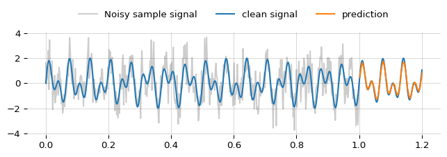
Building a Gaussian process
We can use this autocovariance function to construct a covariance matrix and make a prediction with a conditional Gaussian. I’ve talked about the maths of conditional Gaussians in the appendix of a previous article. Knocking this together looks like:
from scipy.linalg import toeplitz

# Forecast this many steps ahead
horizon = 100

# Turn the autocovariance series into a
# covariance matrix plus a noise term
cov = toeplitz(autocov) + np.eye(N) * 20

# Make a forecast using a conditional
# Gaussian process
AA = cov[:(N-horizon), :(N-horizon)]
BA = cov[(N-horizon):, :(N-horizon)]
forecast = BA @ np.linalg.inv(AA) @ y[horizon:]
Which looks like this:
Summary
You can calculate the autocovariance function of a process from its power spectral density. Using this relationship, here we explored estimating the power spectral density of a noisy time series, calculating its autocovariance matrix and then making a prediction using a conditional Gaussian.