This was a paper I wrote with the intention of publication. I quit academia during the publication process for greener pastures. I’ve published it here myself to save me $2,000 in publisher fees and you in subscription fees.

Introduction

Consider a series of values \(y_i\) that need to be modelled based on some corresponding vectors \(\textbf{x}_i\). One potential family of models for this problem are kernel machines. These are linear models extended into the non-linear world. Generally speaking, a linear model takes a set of points and attempts to find a linear mapping to some specific output. A kernel machine first maps the points into a higher dimension, denoted by \(\varphi(\mathbf{x}_i)\), and then applies a linear algorithm.

Each input vector may be transformed to hundreds of thousands or even an infinite number of dimensions. Mapping each point into this new space is not practical, especially when the embedding space has an infinite number of dimensions. A clever trick is to rearrange the equation for the linear part of the kernel machine so that each input vector is paired with another in a dot product, like so: \(\varphi(\mathbf{x}_i)^T\varphi(\mathbf{x}_j)\). This dot product is usually defined with a simple kernel function. The most common one is the Gaussian kernel which represents the dot product between two points that have been mapped into a space of an infinite number of dimensions: $$ \begin{align} \kappa(\mathbf{x}_i, \mathbf{x}_j) = \varphi(\mathbf{x}_i)^T\varphi(\mathbf{x}_j) = e ^{ - \beta||\mathbf{x}_i - \mathbf{x}_j||^2} \label{1} \end{align} $$ A kernel machine is now a linear model of \(\kappa(\mathbf{x}_i, \mathbf{x}_j)\) instead of \(\mathbf{x}_i\). The book Kernel Adaptive Filtering ¹ discusses different kernel regression models (kernel machine version of linear regression) and provides an easy and detailed mathematical description of how kernel machines work.

The most common kernel machine is the support vector machine (SVM) which has two varieties for modelling classification and regression tasks ^{2 3 4}. SVMs have been used for a wide variety of problems such as pattern recognition ⁵, face recognition ^{6 7}, time series prediction ⁸, image classification ⁹, system control ¹⁰, and function approximation ¹¹.

A common task with SVMs, and kernel machine modeling in general, is tuning the kernel parameters. The most widely used strategy is to conduct cross validation with a separate set of data, which is time consuming. The question we address in this paper is: how to quickly identify an appropriate Gaussian bandwidth parameter \(\beta\) in the Gaussian kernel defined in \(\eqref{1}\)? This parameter is important because it directly affects the geometry of the embedding space. The distance between any two points in this higher dimensional space is: $$ ||\varphi(\mathbf{x}_i) - \varphi(\mathbf{x}_j)||^2 = 2(1 - \varphi(\mathbf{x}_i)^T\varphi(\mathbf{x}_j)) = 2(1 - e ^{ - \beta||\mathbf{x}_i - \mathbf{x}_j||^2}) $$

If \(\beta\) is 0, then each point has zero distance to each other point. If \(\beta \rightarrow \infty\), then each point has exactly a distance of 2 from each other point.

The most common method of selecting \(\beta\) and the parameters to a support vector machine is by a grid search with cross-validation ^{10 12}. Here, every point in a grid of points across the parameter space is tested using cross-validation. This is the most accurate method and the slowest. Typically, evaluating a kernel machine’s prediction error has a complexity on the order of \(O(n^3)\) where \(n\) is the number of data points. A grid search must test a vast number of different parameter values to ensure a high degree of accuracy. One alternative to a grid search is to repeatedly try random points ¹³. However, this does not necessarily reduce the computational burden.

One way to reduce the computational cost is by estimating the error. A large body of literature exists that focuses on estimating an upper bound for the leave-one-out error. Vapnik derives a bound from the number of support vectors ¹⁴ and another bound from the radius of a ball containing all embedded points ²; Jaakkola and Haussler generalises this to kernel machines other than support vector machines ¹⁵; and Opper and Winther applies this bound to SVMs without a threshold ¹⁶. A bounds estimate can be used with a gradient descent algorithm to reduce the number of trials before selecting a set of parameters ¹⁷.

Because the Gaussian kernel’s bandwidth \(\beta\) has a significant effect on the geometry of the embedding space, some algorithms select a value without calculating the prediction error. One study focused on classification tasks and selected the \(\beta\) which maximised the distance between the classes and minimised the distance between points of the same class¹⁸. This algorithm is many times faster than calculating or estimating the model’s error. However, the fitness function is not guaranteed to be convex and thus requires a grid search or a complex search algorithm.

Another study maximised the variance of the distances between data points and found that this idea was fast and comparably accurate ¹². In this paper, we build on this algorithm giving it a significant increase in speed. We show that the selected value for \(\beta\) varies little between small subsets of data. This allows us to confidently use only a small amount of data to find the value for \(\beta\) for a much larger sample set. We also show that these algorithms can be used for both classification and regression tasks.

Solution

We present two methods that select a value for the Gaussian kernel’s bandwidth by focusing on the distance between points.

Consider that if two points are close together, then the value of the Gaussian kernel between these two points will be close to 1. If they are identical, the value will be exactly 1. If, however, the two points are far apart, the value of the Gaussian function approaches 0. We could interpret a value of 1 as meaning the two points are 100% similar, and a value of 0 as meaning they are 0% similar. The Gaussian kernel is then a measure of similarity between two points.

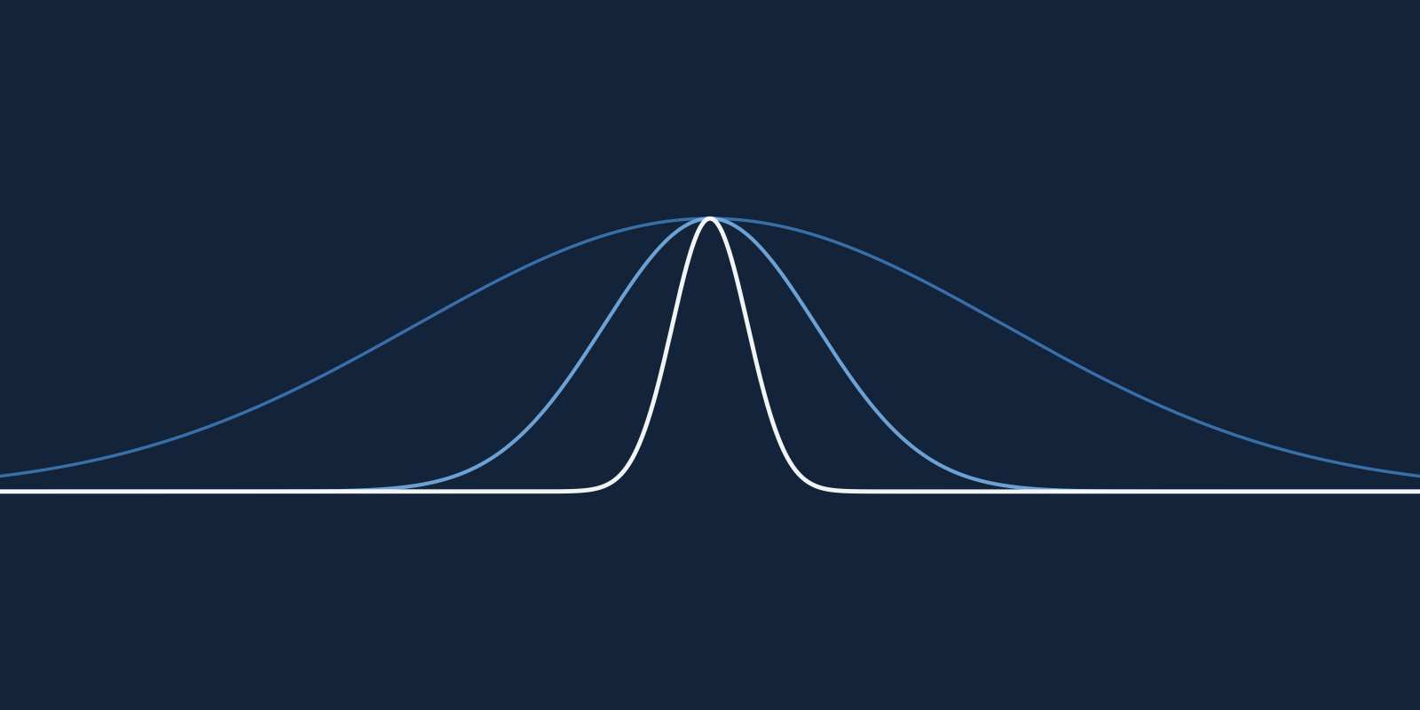
By calculating the similarity between every point in a dataset we get a distribution of similarities. Consider for the moment how this distribution changes as the \(\beta\) parameter of the Gaussian kernel changes. If \(\beta = 0\), then all similarities are equal to one (Figure 1A); all the points are 100% similar. In this situation, a model cannot tell the difference between any points. If \(\beta\) were to grow to \(\infty\), then all similarities are equal to 0 (Figure 1C); all the points are all completely different sharing nothing in common. Now, a model can tell the difference between each point. However, it will not be able to tell which points have something in common. This is where a Gaussian kernel machine should get its power from; the ability to identify how similar a new data point is to previously seen examples. Ideally, then, \(\beta\) ought to be somewhere in-between \(0\) and \(\infty\) (Figure 1B).

Notice in Figure 1B how the similarities are distributed across the entire space from 0 to 1. Some points appear to be similar with a value near 1. Other points have nothing in common with a value near 0. These could be clusters of points that may have predictive power for a target variable. The defining feature here is that the distribution is spread out; relative to other values of \(\beta\), its variance is big. We propose to find a value for \(\beta\) which produces a distribution that is spread out between the two extremes, 0 and 1.

We explore two algorithms in this paper for choosing \(\beta\), the first maximises the similarity distribution’s variance and is called maximum variance, the other optimises the similarity distribution mean called mean-to-half.

Maximum variance

The algorithm propose¹² maximises the Gaussian kernel variance calculated over a training set. The idea is that if this variance is maximised, then the data points will have a wide range of similarities which may help a predictive model identify patterns.

The variance is calculated as: $$ s^2 = \frac{1}{N}\sum_{\forall p} \left( e ^{ - \beta p} - \mu \right)^2 $$

where: $$ \begin{aligned} \mu &= \frac{1}{N}\sum_{\forall p} e ^{ - \beta p} \\ p_{i|j} &= ||\mathbf{x}_i - \mathbf{x}_j||^2 \quad \text{where} \quad i > j, \quad i, j \in [0, …, n] \\ N &= \frac{n(n-1)}{2} \end{aligned} $$

As \(\beta\) increases from \(0\) to \(\infty\) the variance first increases from \(0\) then decreases back to 0 (Figure 2A). The derivative is zero where \(\beta\) maximises the variance (Figure 2B). To the left of the peak, the derivative is above 0, and to the right the derivative is below 0. This allows us to find the value of \(\beta\) that maximises the variance using a binary search. The derivative is: $$ \frac{d}{d\beta}\left[\frac{1}{N}\sum_{\forall p} \left( e ^{ - \beta p} - \mu \right)^2 \right] = -\frac{2}{N}\sum_{\forall p} pe^{-2\beta p} +\frac{2}{N^2}\sum_{\forall p}e ^{ - \beta p}\sum_{\forall p}pe ^{ - \beta p} $$

This derivative is simply a combination of three sums over all the similarities between points in a dataset. If the input vectors have \(m\) dimensions, we can calculate the full time complexity by counting each addition, multiplication and power. The full cost of calculating the derivative at each step is: $$ (3m + 5)\frac{n(n-1)}{2} + \frac{n(n-1)}{2}3 + 1 = O(n^2m) $$

The time complexity of calculating the derivative is \(O(n^2m)\).

Mean-to-half

The previous algorithm directly maximises the similarity variance, however, an indirect method may be faster. We note that the distribution in Figure 1B lies between 0 and 1 with 0.5 as the mid point. If the mean is 0.5 then the variance might be close to its maximum. In this algorithm, we select the value for \(\beta\) where the distribution mean is 0.5.

We calculate the mean similarity as: $$ \mu = \frac{1}{N}\sum_{\forall p} e ^{ - \beta p} $$

As \(\beta\) increases from \(0\) to \(\infty\), the mean decreases because it is a sum of \(e\)s to the power of a negative number (Figure 3). We can find the value for \(\beta\) where the distribution mean is 0.5 using a binary search.

This algorithm runs faster than maximum-variance as it is merely a sum of exponential functions. We calculate the complexity by counting additions, subtractions, multiplications, divisions and powers. If the input vectors have \(m\) dimensions then each similarity is composed of: $$ \frac{n(n-1)}{2} (3m + 1) + \frac{n(n-1)}{2} - 1 + 1 = O(n^2m) $$

The time complexity of calculating the mean is \(O(n^2m)\) and it is faster than the maximum variance algorithm by the amount \(6n(n-1)/2 + 1\).

Results

We test the mean-to-half and maximum variance algorithms on a dataset called SUSY ¹⁹ which describes simulations of particles smashing together in the large hadron collider. The task is to classify whether or not each simulation generated supersymmetric (SUSY) particles. This dataset is discussed in more detail in the Methods section below.

We randomly select 5,000 points from the dataset and evenly split them into a training and test set. We run the mean-to-half algorithm on the training set to find the value for \(\beta\). We then use a grid search with 5-fold cross validation to select the support vector classifier’s regularisation parameter, \(C\). We test \(C\) at 7 evenly spaced values across the range \(10^{-3}\) to \(10^{3}\). We carry out the same analysis with the maximum variance algorithm.

We compare the accuracy of the mean-to-half and maximum variance algorithms against a grid search which represents the best performance and Ahn’s algorithm ¹⁸. The grid search evaluates \(\beta\) at 80 evenly spaced values from \(10^{-3}\) to \(10^{3}\) and the regularising parameter \(C\) at 7 evenly spaced values from \(10^{-3}\) to \(10^{3}\). Ahn’s method checks each value for \(\beta\) in the same set of evenly spaced values and selects the one that maximises the separation between the data classes. We choose \(C\) by performing a grid search at 7 evenly spaced values from \(10^{-3}\) to \(10^{3}\).

We repeat this analysis on four more datasets, Higgs ²⁰ which classes particle simulations as whether or not they produce a Higgs boson; 746 and Impens ²¹ which both classes polyproteins as whether or not they can be split by the HIV-1 protease; and Dress Recommendation ²² which classes dresses in an online shop as whether or not customers recommend them to friends. These datasets are discussed in more detail in the Methods section.

We measure the performance by each method on each dataset by calculating the percentage of correctly predicted outcomes, shown in Figure 4A. We find that both the mean-to-half and maximum variance algorithm perform comparably to the grid search.

The Mashable News Popularity dataset ²³ describes articles published by Mashable including linguistic and topical features. Each article is shared by readers with some being shared more than others. This dataset includes the number of times each article was shared. The task is to estimate how many times an article will be shared before it is published. This is known as a regression task.

In a similar fashion to the previous classification tasks, we randomly select 5,000 points from the completely dataset and split this evenly into a training and test set. We run the mean-to-half algorithm on the training set to find a value for \(\beta\). We then use a grid search with 5-fold cross validation to select the regularisation parameter \(C\) from the same set as we used before and threshold value \(\epsilon\) of a support vector regressor model from a set of 7 evenly spaced between \(10^{-3}\) and \(10^{3}\). We measure the prediction error on the test set by calculating the mean absolute error. We repeat this process using the maximise variance and the grid search algorithms to find the values for \(\beta\) and estimate prediction error. We divide each method’s MAE by the grid search’s MAE to give us the mean absolute percentage error (MAPE) (Figure 4B). We conduct a parallel analysis on two more datasets, Portuguese Students, mathematics class ²⁴ which describes Portuguese students with the aim of predicting their mathematics grades and Portuguese Students, Portuguese class ²⁴ with the aim of predicting their Portuguese grades.

We find that the mean-to-half and maximise variance algorithms perform better than the grid search in all except one example. The maximise variance algorithm performs less than 4% worse than the grid search on the Portuguese mathematics class dataset. We also note from the performance statistics in Figure 4 that these two algorithms are suitable for both classification and regression tasks.

Even though the two algorithms presented here find \(\beta\) faster than others, on large datasets they will still be time consuming. One potential way of dealing with this is to use a small subset of data to find \(\beta\). The problem here is that different subsets may result in a different value for \(\beta\). This approach may only be feasible if \(\beta\) varies little between different subsets.

As a general example, we take 100 random samples of 500 points from the SUSY dataset. For each random sample, we evaluate the mean of the similarity distribution for values of \(\beta\) between \(10^{-2}\) and \(10^{2}\) and depict the squared error from 0.5 in Figure 5A. This is the error function that the mean-to-half algorithm minimises. Each subset is drawn as a grey line with one subset highlighted in blue. For the same random subsets across the same values for \(\beta\) we evaluate the prediction error of a support vector classifier (with \(C = 1/2\)) and show the results in Figure 5B. The best \(\beta\) according to the mean-to-half algorithm appears to vary significantly less than trying to optimise the error.

We quantify this variance by taking 30 random samples of 100 points from the SUSY dataset, finding \(\beta\) with the mean-to-half algorithm on each sample and calculating the variance of \(\beta\)s. We carry out the same analysis with the maximise variance algorithm, Ahn’s algorithm, and a grid search with 5-fold cross validation minimising the prediction error. We repeat this analysis across all the classification datasets. We find that \(\beta\) consistently varies least when using the mean-to-half algorithm and most when using the grid search (Figure 6A). Ahn’s method is not consistent between datasets where it selects the smallest possible \(\beta\) on the Impens dataset and fluctuates between high and low values for \(\beta\) on the remaining dataset.

We repeat this experiment measuring the variance of \(\beta\) as selected by the grid search, maximise variance and mean-to-half algorithms on the regression datasets. Again, we find that the mean-to-half algorithm has the least amount of variance while the grid search has the most (Figure 6B).

Conclusion

In this paper, we propose an algorithm for choosing the Gaussian kernel’s bandwidth parameter which we call mean-to-half. Our work is built on a method propose¹² which we call maximise variance. These two algorithms choose the bandwidth that best highlights clusters of points.

We test these two algorithms on a variety of datasets using support vector machines, both for classification and regression. We find that the algorithms accuracy is comparable to a grid search which represents the best possible result. We also find that the value for \(\beta\) that these two algorithms select is more robust to changes in the dataset than other algorithms. This means that we can find appropriate parameters for large datasets by only examining small subsets.

Our results suggest that we can achieve competitive performance at a greater speed using the maximise variance and mean-to-half algorithms. Our experiments on classification and regression tasks also suggest that these algorithms work independently of the problem to be solved.

These two algorithms can potentially be applied to kernels other than the Gaussian kernel and to kernels with more than one parameter. Such kernels will need to be a measure of similarity and be bounded like the Gaussian kernel.

Methods

In this paper, we explore two algorithms for selecting the bandwidth parameter in kernel machines that use the Gaussian kernel. To test how accurate, robust and versatile these algorithms are, we compare their performance against competing methods for both classification and regression tasks on a number of real world datasets.

Datasets

We use a variety of real-world datasets that cover a wide range of topics such as particle physics, microbiology and education.

SUSY dataset

Physicists at the Large Hadron Collider smash together exotic particles in the hope of detecting supersymmetric (SUSY) particles. These supersymmetric particles are invisible to their detectors and must be inferred from the particles produced by a collision. Two collision are possible; the one we’re interested in called the signal, and a similar collision that does not produce supersymmetric particles called the background noise. The SUSY dataset contains simulations of signal and background collisions. The task is to accurately classify whether each collision produces supersymmetric particles or not. This datasets was used in a study asking whether or not deep learning improves classification ²⁵.

The SUSY dataset contains 5,000,000 simulations. In this study we use a random sample of 5,000 simulations evenly split between the signal and noise records.

Higgs dataset

The Standard Model of particle physics includes a field which gives matter its mass; this is known as the Higgs field. The only means of confirming the existence of the Higgs field is to detect its associated particle, the Higgs boson. Similar to detecting supersymmetric particles, the Large Hadron Collider smashes together particles in the hopes of detecting some Higgs bosons. Just like the SUSY dataset, this dataset lists simulations of collisions and whether or not it produces Higgs bosons. This dataset was used alongside the SUSY dataset in a study asking whether or not deep learning improves detecting Higgs bosons ²⁵.

The Higgs dataset contains 11,000,000 simulations. In this study we use a random sample of 5,000 simulations evenly split between the signal and noise records.

746 dataset

The HIV-1 protease is an enzyme responsible for breaking down certain polyproteins into components of virions that spread HIV. Without this enzyme, the HIV virions are not infectious. Being able to predict which polyproteins the HIV-1 protease breaks down helps scientists test hypotheses of how this enzyme affects the human body. The 746 dataset is a list of polyproteins called octamers which are composed of eight amino acids. The task is to classify whether or not the HIV-1 protease will split an octamer between the fourth and fifth amino acid.

These octamers were collected from various sources in the literature by ²⁶. They were used by ²⁷ to compare the performance of support vector machines with different kernels.

Impens dataset

This dataset is also a list of octamers labelled as split or un-split by the HIV-1 protease. These octamers were collected by ²⁷.

Portuguese Students, mathematics class dataset

To improve understanding of why Portugal’s student failure rate is high, one study collected data from two Portuguese schools ²⁸. The researchers collected data on each student by conducting a survey which asked questions ranging from their romantic relationship to their parent’s alcohol consumption. They also collected the students final grades.

This dataset contains data on students in both schools and their final mathematics grade. The task is to correctly predict their final grade.

Portuguese Students, Portuguese class dataset

As well as the students’ mathematics grades, the study also reports their Portuguese grades. This dataset contains the student’s data and their Portuguese grades. Again, the task is to correctly predict their final grade.

Mashable News Popularity dataset

Mashable is an online news site where readers can share news articles. In one study, researchers collected almost 40,000 articles from Mashable and extracted a set of features from each one including number of positive words, LDA topic distribution and publication time ²⁹. The task is to predict the number of times each article was shared.

The Mashable News Popularity dataset contains 39,797 news articles. In this study we use a random sample of 2,000 simulations evenly split between the signal and noise records.

Support Vector Machines

In this paper, we use support vector machines (SVMs) for both classification and regression tasks. SVMs transform an \(m\) dimensional point into a higher dimension feature space and uses a hyperplane to model the target variable. Denote \(\textbf{x}_i\) and \(y_i\) as the \(i^\text{th}\) input vector and target variable. A SVM transforms these points into a higher dimension but only operates on their dot products. We calculate these dot products with a kernel function: \(\kappa_{\boldsymbol{\theta}}(\textbf{x}_i, \textbf{x}_j)\), where \(\boldsymbol{\theta}\) represents the parameters of the kernel function.

Support vector classification

In a classification problem, the target variable \(y\) is binary and usually denoted \(y \in {-1, 1}\). A support vector classifier (SVC) defines a hyperplane that separates the points into their two classes. The SVCs decision function is: $$ f(\textbf{x}) = \text{sign} \left( \sum_{i = 1}^n \alpha_i y_i \kappa_{\boldsymbol{\theta}}(\textbf{x}_i, \textbf{x}) + b \right) $$

The coefficients \(\alpha\) are found by maximising: $$ \sum_{i=1}^m \alpha_i - \frac{1}{2} \sum_{i,j=1}^m \alpha_i \alpha_j y_i y_j \kappa_{\boldsymbol{\theta}}(\textbf{x}_i, \textbf{x}_j) $$

constrained by: $$ \begin{aligned} & \sum_{i=1}^m \alpha_i y_i = 0 \\ & 0 \leq \alpha_i \leq C, \quad \text{for } i = 1, \dots, m \end{aligned} $$

The constant \(C\) controls the level of over fitting; a large \(C\) leads to an over-fitted model. If the Gaussian function is used as the kernel, then the only parameters are the Gaussian bandwidth \(\beta\) and \(C\). For a deeper explanation of support vector classification see ³ or ².

Support vector regression

In a regression problem, the target variable \(y\) is a real valued scalar. A support vector regressor (SVR) defines a hyperplane as close as possible to all points while ignoring any deviation less than \(\epsilon\). The SVRs function is: $$ f(\textbf{x})= \sum_{i = 1}^n (\alpha_i - \alpha^{\prime}_i) \kappa_{\boldsymbol{\theta}}(\textbf{x}_i, \textbf{x}) + b $$

where the coefficients \(\alpha\) and \(\alpha^{\prime}\) are found by maximising: $$ -\frac{1}{2} \sum_{i,j=1}^m (\alpha_i - \alpha^{\prime}_i) (\alpha_j - \alpha^{\prime}_j)\kappa_{\boldsymbol{\theta}}(\textbf{x}_i, \textbf{x}_j) - \epsilon \sum_{i=1}^m (\alpha_i + \alpha^{\prime}_i) + \sum_{i=1}^m y_i (\alpha_i - \alpha^{\prime}_i) $$

constrained by: $$ \begin{aligned} & \sum_{i=1}^m (\alpha_i - \alpha^{\prime}_i) = 0 \\ & 0 \leq \alpha_i, \alpha^{\prime}_i \leq C, \quad \text{for } i = 1, \dots, m \end{aligned} $$

Similarly to SVCs, the \(C\) term controls the amount of over fitting; a large \(C\) leads to an over-fitted model. If the Gaussian kernel function is used, then there are only three parameters, the Gaussian bandwidth \(\beta\), \(\epsilon\), and \(C\). For a deeper explanation of support vector regression see ⁴ or ².

Finding the bandwidth

Grid search

The simplest way to select a kernel machine’s parameters is to evaluate it’s prediction error for a range of parameters and select the best ones. The general approach is to form a grid of evenly spaced points across some range of the parameter space, hence the name grid search. For each set of parameters we use a 5-fold cross validation to estimate the error on a training set.

To find a suitable value for the Gaussian bandwidth, we must perform a grid search across all the model’s parameters because we have to evaluate the error. For a support vector classifier the only other parameter is the regularisation term \(C\), and for a support vector regressor it is the threshold term \(\epsilon\).

Ahn’s method

A study conducted by Ahn looks at classification problems and choose a kernel’s parameters by minimising the average distance between points of the same class and maximising the average distance between points of different classes ¹⁸.

If we represent \(\textbf{x}_i\) and \(\textbf{y}_j\) to be vectors of two difference classes, we can write the mean distance between vectors of the same class as:

$$ \begin{aligned} & \frac{1}{2} \left( \frac{1}{m^{(T)}} \sum^m_{i,j=1; i > j} ||\varphi(\textbf{x}_i) - \varphi(\textbf{x}_j)||^2 + \frac{1}{n^{(T)}} \sum^n_{i,j=1; i > j} ||\varphi(\textbf{y}_i) - \varphi(\textbf{y}_j)||^2 \right) \\ &= \frac{1}{2} \left( \frac{1}{m^{(T)}} \sum^m_{i,j=1; i > j} \kappa(\textbf{x}_i, \textbf{x}_j) + \frac{1}{n^{(T)}} \sum^n_{i,j=1; i > j} \kappa(\textbf{y}_i, \textbf{y}_j) \right) \end{aligned} $$

where \(m\) is the number of points in the first class, and \(n\) the number of points in the second class and \(a^{(T)} = a(a-1)/2\) is the number of distances between \(a\) points. The mean distance between vectors of different classes as: $$ \frac{1}{mn}\sum^m_{i=1}\sum^n_{j=1} ||\varphi(\textbf{x}_i) - \varphi(\textbf{y}_j)||^2 = \frac{1}{mn}\sum^m_{i=1}\sum^n_{j=1} \kappa(\textbf{x}_i, \textbf{y}_j) $$

Ahn suggests that a good choice of the kernel parameters maximises the difference between the within distance and distance between points of different classes: $$ \frac{1}{m^{(T)}} \sum^m_{i,j=1; i > j} \kappa(\textbf{x}_i, \textbf{x}_j) +\frac{1}{n^{(T)}} \sum^n_{i,j=1; i > j} \kappa(\textbf{y}_i, \textbf{y}_j) - \frac{2}{mn}\sum^m_{i=1}\sum^n_{j=1} \kappa(\textbf{x}_i, \textbf{y}_j) $$

Similar to the two methods proposed in this paper (maximum variance and mean-to-half) this method is a linear combination of the Gaussian similarity between each point. Ahn demonstrated that the global maximum is robust to changes in the data. However, this function also has local maxima which prevents a fast search algorithm.

Appendix

Complexity of maximum variance

Each similarity is composed of:

• \(m\) subtractions, \(m\) powers and \(m-1\) additions: \(p = ||\textbf{x}_i - \textbf{x}_j||^2\)
• 2 multiplications: \(-2 \beta p\), \(\beta p\)
• 2 powers: \(e^{-2 \beta p}\), \(e^{\beta p}\)
• 2 multiplications: \(p e^{-2 \beta p}\), \(e^{\beta p}\), \(p e^{\beta p}\)

In total, each similarity costs \(3m + 5\) operations, and there are \(n(n-1)/2\) similarities resulting in \(3m + 5)n(n-1)/2\) operations. Then, these similarities are summed together and combined to form the derivative:

• \((\frac{n(n-1)}{2} -1) \times 3\) additions: \(\sum_{\forall p}p e^{-2 \beta p}\), \(\sum_{\forall p}e^{\beta p}\), \(\sum_{\forall p}p e^{\beta p}\)
• 3 multiplications: \(-\frac{2}{N}\sum_{\forall p}p e^{-2 \beta p}\), \(\frac{2}{N^2}\sum_{\forall p}e^{\beta p} \sum_{\forall p}p e^{\beta p}\)
• 1 addition: \(-\frac{2}{N}\sum_{\forall p}p e^{-2 \beta p} + \frac{2}{N^2}\sum_{\forall p}e^{\beta p} \sum_{\forall p}p e^{\beta p}\)

This step has a total cost of \(\frac{n(n-1)}{2}3 + 1\) operations. The full cost of calculating the derivative at each step is: $$ \begin{aligned} (3m + 5)\frac{n(n-1)}{2} + \frac{n(n-1)}{2}3 + 1 &= \frac{n(n-1)}{2} (3m + 8) + 1 \\ &= O(n^2m) \end{aligned} $$

Complexity of mean to half

We expect that this algorithm ought to run faster than maximum-variance as this is merely a sum of exponential functions. We calculate the complexity by counting additions, subtractions, multiplications, divisions and powers. If the input vectors have \(m\) dimensions then each similarity is composed of:

• \(m\) subtractions, \(m\) powers and \(m-1\) additions: \(p = ||\textbf{x}_i - \textbf{x}_j||^2\)
• 1 multiplication: \(-\beta p\)
• 1 exponential: \(e^{\beta p}\)

Thus a single Gaussian kernel functions takes \(3m + 1\) operations to calculate. If there are $n$ data points then there are \(\frac{n(n-1)}{2}\) distances. We need to calculate each distance, add them together and divide by the number of distances: $$ \begin{aligned} \frac{n(n-1)}{2} (3m + 1) + \frac{n(n-1)}{2} - 1 + 1 &=\frac{n(n-1)}{2}[3m + 2] \\ & = O(n^2m) \end{aligned} $$

Footnotes

References & Notes

Corrections

If you see any mistakes or room for improvement, please reach out to me on Twitter @DrAdrian.

Citation

Please cite this work as:

Letchford (2015), "Choosing the Gaussian Kernel's Bandwidth", OS Quant.

In BibTeX please use:

@article{Letchford2015,
    author = {Letchford, Adrian},
    title = {Choosing the Gaussian Kernel's Bandwidth},
    journal = {OS Quant},
    year = {2015},
    note = {https://osquant.com/papers/choosing-the-guassian-kernal-bandwidth/},
}