Like what you see? Follow Adrian on Twitter to be notified of new content. Follow

This was a paper I wrote with the intention of publication. I quit academia during the publication process for greener pastures. I’ve published it here myself to save me $2,000 in publisher fees and you in subscription fees.

Introduction

Consider a series of continuous values $y_i$ that need to be modelled based on some corresponding vectors $\textbf{x}_i$. A model that is potentially suitable for this task is called the support vector regression model. This maps the points $\textbf{x}_i$ into a higher dimension denoted by $ \varphi(\mathbf{x}_i) $, and then models $y_i$ by fitting a linear model based on a subset of $\textbf{x}$ called support vectors.

Support vector regression models are part of a branch of models called support vector machines (SVM) ¹ ² ³. SVMs have been used for a wide variety of problems such as pattern recognition ⁴, face recognition ⁵ ⁶, time series prediction ⁷, image classification ⁸, system control ⁹, and function approximation ¹⁰.

Support vector regression is a powerful model because each input vector may be transformed into an extremely high number of dimensions. This transformation is rarely computationally efficient. However, the model’s equations can be rearranged so that each transformed vector is paired with another in a dot product, like so: $\varphi(\mathbf{x}_i)^T\varphi(\mathbf{x}_j)$. This dot product is usually defined with a simple kernel function. The most common one is the Gaussian kernel:

$$ \begin{align} \kappa(\mathbf{x}_i, \mathbf{x}_j) = \varphi(\mathbf{x}_i)^T\varphi(\mathbf{x}_j) = e ^{ - \beta||\mathbf{x}_i - \mathbf{x}_j||^2} \label{1} \end{align} $$

A necessary task when fitting a support vector regression (SVR) model is tuning the kernel parameters. The most common method of selecting $\beta$ in $\eqref{1}$ and the parameters to a SVR is by a grid search with cross-validation ⁹ ¹¹. In a grid search, the parameter space is divided into a grid of points where each one is tested using cross-validation. Given a vast number of grid points, this is the most accurate method. Evaluating a SVR model’s prediction error has a complexity on the order of $O(n^3)$ where $n$ is the number of data points. This cubic complexity makes the grid search the slowest method. Various alternatives do not necessarily work around the evaluation complexity. For example, one alternative is to test random points rather than use a grid ¹².

In this paper, I develop an algorithm to find a value for $\beta$ from a set of training points. This algorithm does not calculate the model’s prediction error and runs in $O(n^2)$ time. The resulting error is just as good as an exhaustive grid search. I show that, on some datasets, the selected value for $\beta$ varies considerably between small subsets of data; which means that this algorithm can sometimes trade robustness for the improvement in speed.

Finding the Gaussian kernel parameter

This method selects a value for the Gaussian kernel’s bandwidth by focusing on the distance between the output values $y$. A kernel machine models the target value $y$ as a function of the dot product between the input vectors $x$. The dot product can be thought of as a measure of similarity between two vectors. The algorithm presented here attempts to select values for a kernel’s parameters so that two $x$ vectors are more similar if their corresponding $y$ values are also similar.

**Figure 1: An example time series.** In this example, $y = \sin(x) + \sin(3x) + \sin(2x + 5)$.

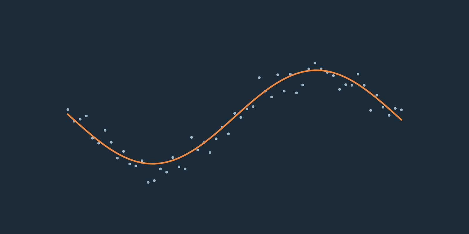
Consider the example time series in Figure 1. In this example, we want to predict the next value in this series based on the last 20 values. The last 20 values at time $t$ can be represented as $\textbf{x}_t$ and the target value as $y_t$. The Gramian matrix, sometimes known as the feature matrix, is a matrix of dot products between each of the $\textbf{x}$ vectors. This is written as $\textbf{K}$: $$ \begin{aligned} \textbf{K} = \left[\begin{matrix} \kappa(\textbf{x}_0, \textbf{x}_0) & \dots & \kappa(\textbf{x}_0, \textbf{x}_n) \\ \vdots & \ddots & \vdots \\ \kappa(\textbf{x}_n, \textbf{x}_0) & \dots & \kappa(\textbf{x}_n, \textbf{x}_n) \end{matrix} \right] \end{aligned} $$

For the example time series, the Gramian matrix with the Gaussian kernel is shown in Figure 2A. The value for $\beta$ was chosen by hand and is not important in this example. Observe in Figure 2B what happens after sorting the vectors by their $y$ values in an ascending order. Now, adjacent $\textbf{x}$ vectors have a close value for their corresponding target $y$. Notice that cells close to the main diagonal are red (value close to 1), and the further a cell is from the diagonal the more blue (value close to 0) it is.

**Figure 2: The Gramian matrix of the time series in Figure 1.** **(A)** Consider the problem of predicting the next value of the example series in Figure 1 using the previous 20 values. The value at time $t$ is represented with $y_t$ and the previous 20 with $x_t$. Here you can see the Gramian matrix where each cell is the value of the Gaussian function between two $x$ vectors. The bandwidth parameter was chosen to highlight the pattern, its exact value is not important. **(B)** If the $x$ vectors are sorted by their corresponding target value $y$, the pattern is destroyed, however, a new pattern emerges. Now, values closer to the main diagonal are more red. That is, the kernel function of two $x$ vectors tends to be closer to 1 when their corresponding $y$s are closer in value.

Now that the vectors are sorted, the further away a cell is from the main diagonal, the more distant their target values. Ideally, just like in Fig. 2B, we want the $\textbf{x}$ vectors that correspond to the cells to also be less similar. We can visualise this decrease in similarity by taking the mean value of each of the matrix’s lower diagonals. We can ignore the upper diagonals because they are exactly the same–a Gramian matrix is symmetric. In Figure 3 we plot the mean of each of the diagonals in Fig. 2B. Again we can see that the kernel function’s values are more similar when closer to the main diagonal. In this example, the average value decreases to zero the further from the main diagonal.

**Figure 3: Mean of the Gramian diagonals.** **(A)** Using the sorted Gramian matrix in Figure 2B, we plot the mean of each diagonal. The first value on the left hand side is the first diagonal from the center. The last value is the cell in the lower left hand corner of the Gramian matrix. Diagonals closer to the center represent vectors that are closer together. Here we see that the mean of each diagonal decreases farther from the center. This suggests that when multiple $y$s are close together, their corresponding $x$ vectors are also close. **(B)** We repeat the analysis in (A) with the exception of adding some Gaussian noise to the example time series. The least amount of noise is shown in blue and the most amount of noise is shown in red. This suggests that as noise is added to the data, $x$ vectors are no longer close when their corresponding $y$ values are close. We propose that the slope of this line may be a good indicator that the $x$ vectors describe the $y$ values.

If we add noise to the time series in Figure 1 and calculate the mean of each of the Gramian’s diagonals, then this line becomes flatter and more erratic as more noise is added (Figure 3B). The slope of the mean diagonal line seems to be a crude measure of how the similarity between the $\textbf{x}$ vectors match the similarity between the $y$ values.

The algorithm in this paper chooses $\beta$ such that the slope of this line is as negative as possible. For lack of a better name, we call this the diagonal slope algorithm.

Diagonal Slope Algorithm

We calculate the slope by taking the difference between each successive diagonal mean. These are then combined together in a weighted average to find the average slope. The weights are chosen to be the total number of cells in the corresponding diagonals.

Calculating the mean of each diagonal does not require us to compute the whole Gramian matrix. The main diagonal contains only 1, and the matrix is symmetric. This means we only need the upper or lower triangle of this matrix. Here, our notation will use the lower triangle:

$$ \begin{aligned} K = \left[\begin{matrix} 1 \\ \kappa(\textbf{x}_1, \textbf{x}_0) & 1 \\ \vdots & \vdots & \ddots & 1 \\ \vdots & \vdots & \vdots & \ddots & \ddots \\ \kappa(\textbf{x}_n, \textbf{x}_0) & \dots & \dots & \dots & \kappa(\textbf{x}_n, \textbf{x}_{n-1}) & 1 \end{matrix}\right] \end{aligned} $$

For simplicity’s sake, we’ll denote each cell with a single index instead of two, and refer to them with $p$: $$ \begin{aligned} K &= \left[\begin{matrix} 1 \\ p_0 & 1 \\ p_1 & p_{n-1} & 1 \\ p_2 & p_{n} & \ddots & 1 \\ \vdots & \vdots & \vdots & \ddots & \ddots \\ p_{n-2} & \dots & \dots & \dots & p_{n(n-1)/2} & 1 \end{matrix}\right] \\ p_i &= \kappa(\textbf{x}_{\text{row}(i)}, \textbf{x}_{\text{col}(i)}) \\ \text{row}(i) &= \text{col}(i) + \text{diag}(i) + 1 \\ \text{col}(i) &= \Bigg\lfloor{\frac{(2n - 1) - \sqrt{(2n - 1)^2 - 4 \cdot 2i}}{2}}\Bigg\rfloor \\ \text{diag}(i) &= i - - \frac{- (2n-1)\text{col}(i) + \text{col}(i)^2}{2} \end{aligned} $$ The functions $\text{col}(i)$, $\text{row}(i)$, $\text{diag}(i)$ give the column, row, and diagonal index of a cell $i$ respectively. The functions are derived in the appendix.

Ignoring the main diagonal of ones, there are $n-2$ diagonals which we denote with $d$. The zeroth mean diagonal is: $$ d_0 = \frac{p_0 + p_{n-1} + \dots + p_{n(n-1)/2}}{n-1} $$

and the $j^{\text{th}}$ diagonal is: $$ d_j = \frac{1}{n-2-j+1} \sum_{i=0}^{n-2-j} p_{in-i(i+1)/2+j} $$

We calculate the slope by taking the weighted average of the differenced mean diagonal line:

$$ \begin{aligned} S &= \frac{ \frac{d_1 -d_0}{l_1+l_0} + \frac{d_2 -d_1}{l_2+l_1} + \dots }{ (l_1 + l_0) + (l_2 + l_1) + \dots } \\ &= \frac{ -d_0(l_0 + l_1) + \sum_{i=1}^{n-3} d_i(l_{i-1} - l_{i+1}) + d_{n-2}(l_{n-2} + l_{n-3}) }{ l_0+2\sum_{i=1}^{n-3}l_i + l_{n-2} } \end{aligned} $$

This is a linear combination of $p$s and we can write it as such: $$ \begin{align} S = \sum_{i=0}^{n(n-1)/2} w_i p_i \label{2} \end{align} $$

Each weight is calculated as:

$$ w_i^* = \frac{1}{n-2-\text{diag}(i)+1} \times \frac{1}{l_0+2\sum_{j=1}^{n-3}l_j + l_{n-2}} $$ $$ \begin{align} w_i &= \begin{cases} -w_i^*(l_0 + l_1), & \text{if}\ \text{diag}(i)= 0 \\ -w_i^*(l_{\text{diag}(i)-1} - l_{\text{diag}(i)+1}), & \text{if}\ 1 \geq \text{diag}(i) \geq n-3 \\ w_i^*(l_{n-2} + l_{n-3}), & \text{if}\ \text{diag}(i)= n-2 \end{cases} \label{3} \end{align} $$

The objective function $\eqref{2}$ is shown in Figure 4A using the time series example in Figure 1.

**Figure 4: Examples of the objective function.** **(A)** The objective function on the example time series in Figure 1. **(B)** The objective function on a randomly generated time series shows that there is no guarantee that it will be convex.

All weights in the objective function $\eqref{2}$ are positive except for when $\text{diag}(i)= 0$ $\eqref{3}$. As a result, there is no guarantee that the objective function $\eqref{2}$ has a single minima. Figure 4B shows an example of the objective function when the time series values are drawn from a Gaussian distribution. Because the objective function is not guaranteed to have a single minima, we use an exhaustive search to find the global minima in this paper.

Results

We use a dataset called the Mashable News Popularity dataset ¹³ to evaluate the diagonal slope algorithm described in the previous section. This dataset is a collection of features on 2,000 articles from the online news site Mashable. The task is to predict the number of times each article is shared. We provide a full description of this dataset in Appendix 2.

We randomly split this dataset into two even subsets, one for training and one for testing. We convert any non-numeric dimensions into an orthogonal representation. We normalise the training dataset by subtracting the mean from each dimension and dividing by their standard deviations. We normalise the testing dataset using the same mean and standard deviation.

We evaluate the diagonal slope algorithm’s objective function for each $\beta$ from $10^{-3}$ to $10^{3}$ at $80$ logarithmic evenly spaced values. After finding the $\beta$ which minimises the diagonal slope, we use a grid search to fit the $\epsilon$ and $C$ parameters of a support vector regressor. We evaluate $\epsilon$ at 5 logarithmic evenly spaced values from $10^{-3}$ to $10^1$, and $C$ at 7 logarithmic evenly spaced values from $10^{-3}$ to $10^{3}$.

We find that the support vector regressor fitted with the diagonal slope algorithm has a mean absolute error (MAE) of 0.30 on the testing data while the plain grid search’s MAE is also 0.30. These results show that our algorithm achieves a comparable forecasting error with an exhaustive grid search but at a fraction of the time.

We verify this result by performing the same analysis on six other datasets. We use a dataset for predicting Portuguese student’s mathematics grades ¹⁴, predicting Portuguese student’s Portuguese grades ¹⁵, classifying the age of a song ¹⁶, predicting housing prices in Boston ¹⁷, predicting the number of comments on blog posts ¹⁸, and predicting the number of bicycles rented in a bike-sharing system ¹⁹. Again, we provide a full description of each of the datasets in Appendix 2.

**Figure 5: The error is just as good as the standard slow and exhaustive method.** The dataset *Mashable News Popularity* is a collection of articles from the news website Mashable and the aim is to predict the the number of times each article is shared based on a set of features. We randomly split this dataset evenly into a training and testing set. We train the proposed diagonal slope algorithm and a basic grid search on the training sample and evaluate the mean absolute percentage error (MAPE) on the testing set. We repeat this process on the remaining datasets. We find that the error from the diagonal slope algorithm is never more than 5% greater than the grid search.

The results are shown in Figure 5. While the diagonal slope algorithm’s error is slightly higher or lower on some datasets, it is never greater by more than 5%. These results suggest that our algorithm does not trade accuracy for speed.

Because kernel algorithms can be slow when using large datasets, a common practice is to fit a model on a small subset. However, there is a possibility that an algorithm for choosing the kernel parameters is sensitive to the subset. If the subset changes, the selected parameters might also change quite significantly. An algorithm that is able to choose consistent kernel parameters is called robust.

To check whether or not our algorithm is more or less robust than the grid search, we draw with replacement 30 random subsets of 100 points from each datasets. We use the diagonal slope algorithm and grid search to find a suitable value for $\beta$ on each subset. We then compare the variance of the $\beta$s as chosen by the two algorithms.

**Figure 6: The proposed algorithm is not always robust.** We take 30 random samples of 100 articles from the *Mashable News Popularity* dataset. We fit both the diagonal slope algorithm and a basic grid search to each of the samples and record the fitted $\beta$. We then calculate the variance between the selected values. Here we show that the value for $\beta$ selected by the diagonal slope algorithm has a greater variance than if selected by the grid search. We repeat this analysis on all the data sets and find that the diagonal slope algorithm’s variance is greater for three of the datasets. This demonstrates that the proposed algorithm is not always robust.

We show the variance of the $\beta$s in Figure 6. On three data sets, the diagonal slope algorithm has a greater variance than the grid search. We conclude that the diagonal slope algorithm is not always as robust as a grid search.

Summary

In this paper, I propose an algorithm for choosing kernel parameters in regression tasks termed the diagonal slope algorithm.

This algorithm was tested on a variety of datasets using the Gaussian kernel and support vector regression. The algorithm’s accuracy is comparable to a grid search which represents the best possible result. However, the algorithm’s choice of the Gaussian kernel’s bandwidth parameter is sometimes sensitive to changes in the training data.

These results suggest that the speed gained from using the diagonal slope algorithm does not reduce performance, but it does sometimes reduce robustness. This algorithm can potentially be applied to kernels other than the Gaussian kernel and to kernels with more than one parameter. Such kernels will need to be a measure of similarity or be normalised. A normalised kernel represents the correlation of two points in feature space.

Appendices

Appendix 1 - Row and column indices of a matrix cell

A Gramian matrix is a matrix of the dot products between a set of vectors. The matrix is symmetric and the values along the main diagonal are identical because they correspond to the dot product between two identical points. The only unique values in a Gramian matrix are in the upper or lower triangle. Here, we will use the lower triangle.

**Figure 7: Matrix indexing.** Because a Gramian marix is symmetric and the diagonals are all the same value we only need to index the lower triangle. Here, we depict how each cell is indexed with a top to bottom approach. The indexes for the columns, rows and diagonals are also shown.

We can index each cell in the lower triangle of a Gramian matrix as shown in Figure 7 which represents the matrix made by 6 vectors. In this appendix, we derive the column, row and diagonal index from the cell index.

We represent the cell index with $i$ and the total number of vectors which produce the Gramian matrix with $n$. First we figure out the function $\text{col}(i)$ which calculates the column index. Given a column index $c$, the $i$ that sits at the top of that column is: $$ i = \frac{n(n-1)}{2} - \frac{(n - c)(n - c-1)}{2} $$

We can factor this down to: $$ %i &= n^{(T)} - (n - c)^{(T)} \ %i &= n^{(T)} - \frac{(n-c)(n-c-1)}{2} \ %i &= n^{(T)} - \frac{n^2 - n - (2n-1)c + c^2}{2} \ %i - n^{(T)} &= - \frac{n^2 - n - (2n-1)c + c^2}{2} \ %i - n^{(T)} + n^{(T)} &= -\frac{- (2n-1)c + c^2}{2} \ i = -\frac{- (2n-1)c + c^2}{2} $$

and solve for $c$: $$ \begin{aligned} %2i &= - (2n-1)c + c^2 \ %0 &= - (2n-1)c + c^2 - 2i \ c &= \frac{(2n - 1) \pm \sqrt{(2n - 1)^2 - 4 \cdot 2i}}{2} \\ c &= \frac{(2n - 1) - \sqrt{(2n - 1)^2 - 4 \cdot 2i}}{2} \end{aligned} $$

For any $i$ that does not sit at the top of a column, $c$ will be between the column index and the next column’s index. We have to floor this value to get the column index of $i$: $$ \text{col}(i) = \Bigg\lfloor\frac{(2n - 1) - \sqrt{(2n - 1)^2 - 4 \cdot 2i}}{2}\Bigg\rfloor $$

The diagonal is the number of spaces the $i$ sits from the top of it’s column: $$ \text{diag}(i) = i - - \frac{- (2n-1)\text{col}(i) + \text{col}(i)^2}{2} $$

The row is the column plus the diagonal: $$ \text{row}(i) = \text{col}(i) + \text{diag}(i) + 1 $$

Appendix 2 - Datasets

We use a variety of real-world datasets that cover a wide range of topics such as micro-blogging and education.

Mashable News Popularity dataset

Mashable is an online news site where readers can share news articles. In one study, researchers collected almost 40,000 articles from Mashable and extracted a set of features from each one including number of positive words, LDA topic distribution and publication time ²⁰. The task is to predict the number of times each article was shared.

The Mashable News Popularity dataset ¹³ contains 39,797 news articles. In this study we use a random sample of 2,000 articles.

Portuguese Students, mathematics class dataset

To improve understanding of why Portugal’s student failure rate is high, one study collected data from two Portuguese schools ²¹. The researchers collected data on each student by conducting a survey which asked questions ranging from their romantic relationship to their parent’s alcohol consumption. They also collected the students final grades.

This dataset ¹⁴ contains data on 395 students in both schools and their final mathematics grade. The task is to correctly predict their final grade.

Portuguese Students, Portuguese class dataset

As well as the students’ mathematics grades, the study also reports their Portuguese grades. This dataset contains data on 649 students and their Portuguese grades. Again, the task is to correctly predict their final grade.

Million Song

This dataset ¹⁶ is a collection of 515,245 songs selected from the Million Song Dataset ²². It contains 90 attributes for each song which are the means and covariances of the timbre across segments within a song. The task is to predict the year each song was produced. In this study we use a random sample of 2,000 songs.

Housing

This is a dataset of 506 houses in Boston and their prices as used by ²³. The task is to predict the median housing price from a set of features which includes crime rate, average number of rooms, tax rates and socio-economic states.

Blog Feedback

This is a dataset of 60,000 blog posts from around 1,200 Hungarian blogs. It has 280 recorded features for each post including number of links, number of comments received thus far and the most discriminative features from a bag of words analysis. The goal is to predict the number of comments each post will receive in the next 24 hours. This dataset was used by ²⁴. We use a random subset of 2,000 blog posts.

Bike sharing systems completely automate the rental and return process of renting bikes. Users are able to rent a bike from one location, and return the bike to another. This dataset contains daily records of a bike-sharing system called Capital Bike Sharing in Washington, D.C., USA. It has two years of records from the 1^st of January 2011 to the 31^st of December 2012 for a total of 731 days. This dataset was used by ²⁵ to test an event detection algorithm. In this paper, the task is to predict the number of rented bikes from the day’s weather records.

Like what you see? Follow Adrian on Twitter to be notified of new content. Follow

Footnotes

References & Notes

Vapnik, Vladimir: “Statistical learn theory” Wiley & Sons New York (1998) ↩︎
Burges, Christopher J C: “A tutorial on support vector machines for pattern recognition” Data Mining and Knowledge Discovery 2(2) pp. 121–167 Springer (1998) ↩︎
Smola, AlexJ. and Schölkopf, Bernhard: “A tutorial on support vector regression” Statistics and Computing 14(3) pp. 199–222 Kluwer Academic Publishers (2004) ↩︎
Wang, Tai-Yue and Chiang, Huei-Min: “Fuzzy support vector machine for multi-class text categorization” Information Processing & Management 43(4) pp. 914–929 Kluwer Academic Publishers (2007) ↩︎
Phillips, P Jonathon: “Support Vector Machines Applied to Face Recognition” Proceedings of the 1998 Conference on Advances in Neural Information Processing Systems II pp. 803–809 MIT Press Cambridge, MA, USA (1999) ↩︎
Li, S Z and Fu, QingDong and Gu, Lie and Scholkopf, Bernhard and Cheng, Yimin and Zhang, Hongjiag: “Kernel machine based learning for multi-view face detection and pose estimation” Computer Vision, 2001. ICCV 2001. Proceedings. Eighth IEEE International Conference on 2 pp. 674–679 MIT Press Cambridge, MA, USA (2001) ↩︎
Kim, Kyoung-jae: “Financial time series forecasting using support vector machines” Neurocomputing 55(1-2) pp. 307–319 (2003) ↩︎
Chapelle, O and Haffner, P and Vapnik, V N: “Support vector machines for histogram-based image classification” Neural Networks, IEEE Transactions on 10(5) pp. 1055–1064 (1999) ↩︎
Hong, X and Chen, S and Gao, J and Harris, C J: “Nonlinear Identification Using Orthogonal Forward Regression With Nested Optimal Regularizationn” Neural Networks, IEEE Transactions on PP(99) pp. 1 (2015) ↩︎ ↩︎
Vapnik, Vladimir and Golowich, Steven E and Smola, Alex: “Support Vector Method for Function Approximation, Regression Estimation, and Signal Processing” Advances in Neural Information Processing Systems 9 pp. 281–287 MIT Press Cambridge, MA, USA (1996) ↩︎
Tang, Yaohua Tang Yaohua and Guo, Weimin Guo Weimin and Gao, Jinghuai Gao Jinghuai: “Efficient model selection for Support Vector Machine with Gaussian kernel function” IEEE Symposium on Computational Intelligence and Data Mining pp. 40-45 (2009) ↩︎
Bergstra, James and Bengio, Yoshua: “Random Search for Hyper-Parameter Optimization” Journal of Machine Learning Research 13 pp. 281–305 (2012) ↩︎
Online news popularity dataset ↩︎ ↩︎
Student performance, mathematics dataset ↩︎ ↩︎
Student performance, Portuguese dataset ↩︎
Million song dataset ↩︎ ↩︎
House prices dataset ↩︎
Blog feedback dataset ↩︎
Bike sharing dataset ↩︎
Fernandes, K. and Vinagre, P. and Cortez, P.: “A Proactive Intelligent Decision Support System for Predicting the Popularity of Online News” Proceedings of the 17th EPIA 2015 - Portuguese Conference on Artificial Intelligence Coimbra, Portugal (2015) ↩︎
Cortez, Paulo and Silva, Alice: “Using Data Mining To Predict Secondary School Student Performance” In the Proceedings of 5th Annual Future Business Technology Conference 2003(2000) pp. 5–12 MIT Press A. Brito and J. Teixeira (2008) ↩︎
Bertin-Mahieux, Thierry and Ellis, Daniel P W and Whitman, Brian and Lamere, Paul: “The Million Song Dataset” Proceedings of the 12th International Conference on Music Information Retrieval (2011) ↩︎
Quinlan, J R: “Combining Instance-Based and Model-Based Learning” Proceedings of the Tenth International Conference of Machine Learning pp. 236–243 Morgan Kaufmann (1993) ↩︎
Buza, Krisztian: “Feedback Prediction for Blogs” Data Analysis, Machine Learning and Knowledge Discovery SE - 16 pp. 145–152 Springer International Publishing (2014) ↩︎
Fanaee-T, Hadi and Gama, Joao: “Event labeling combining ensemble detectors and background knowledge” Progress in Artificial Intelligence 2(2-3) pp. 113–127 Springer Berlin Heidelberg (2014) ↩︎

Corrections

If you see any mistakes or room for improvement, please reach out to me on Twitter @DrAdrian.

Citation

Please cite this work as:

Letchford (2016), "Fast Gaussian Kernel fit for Support Vector Regression", OS Quant.

In BibTeX please use:

@article{Letchford2016,
    author = {Letchford, Adrian},
    title = {Fast Gaussian Kernel fit for Support Vector Regression},
    journal = {OS Quant},
    year = {2016},
    note = {https://osquant.com/papers/fast-guassian-kernel-fit-for-support-vector-regression/},
}