Like what you see? Follow Adrian on Twitter to be notified of new content. Follow

This write up is my notes on a few papers looking at using order book data to model price movements.

Volume imbalance

The key idea when analysing the limit order book is to identify whether the market as a whole is leaning more towards buying or selling. This idea is call volume imbalance.

Volume imbalance at time $t$ is defined as ¹ ² ³: $$ \rho_t = \frac{V_t^b - V_t^a}{V_t^b + V_t^a}, \ \ -1 \leq \rho_t \leq 1 $$ where $V_t^b$ is the volume at time $t$ posted at the best bid and $V_t^a$ the volume at the best ask. We can interpret a $\rho_t$ close to 1 as signalling strong buying pressure and a $\rho_t$ close to -1 as strong selling pressure. This only takes into account the volume posted at the best bid and ask, the L1 order book.

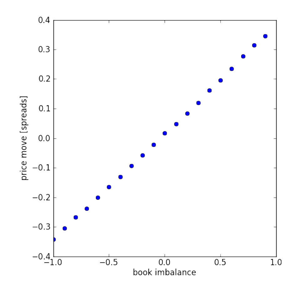
Lipton et. al. ² compared the price imbalance with the subsequent price normalised by the spread. The following figure is copied from their paper:

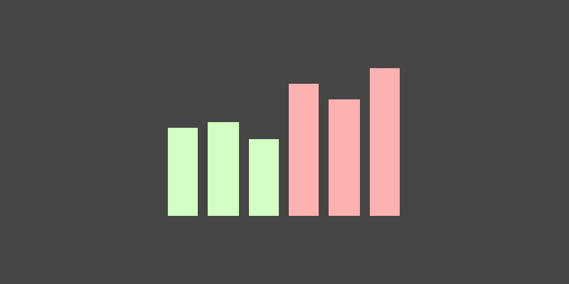
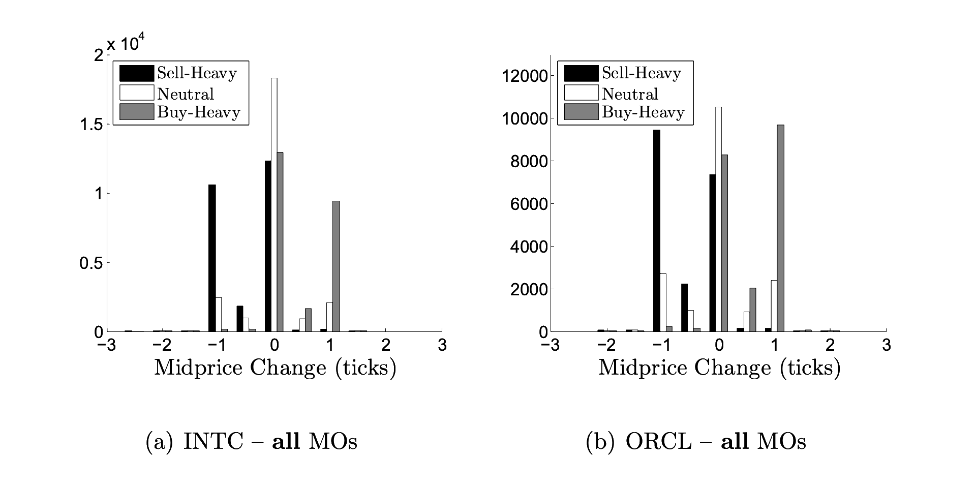
**Volume imbalance vs price move.** This figure shows the bucketed volume imblanace (x axis) vs the average future price move normalised by the spread (y axis). The dataset is the flow of orders for Vodafone (VOD.L) during the first quarter of 2012. There appears to be a linear relationship between the level 1 order imbalance and future price moves. However, on average, the future price move is within the bid-ask spread.

A key paper split the volume imbalance $\rho_t$ into the following three segments ¹:

Interval	Label
$-1 \geq \rho_t \gt -\frac{1}{3} $	Sell-heavy
$-\frac{1}{3} \geq \rho_t \geq \frac{1}{3} $	Neutral
$\frac{1}{3} \gt \rho_t \geq 1 $	Buy-heavy

The authors found that these segments predicted future price moves. The following figure is copied from their paper:

**Predictive power of volume imbalance.** **(a)** The tick by tick order book for Intel (INTC) was analysed over the period January 2014 to December 2014. For each arriving market order (MO), the volume imbalance was recorded and segmented with the number of ticks that the mid price changed by over the next 10 milliseconds. The chart shows the distribution of segments & mid price changes. We can see that positive price moves are more likely to have been preceded by a buy-heavy order book. Similarly, negative changes are more likely to have been preceded by a sell-heavy book. **(b)** These results are replicated for Oracle (ORCL).

Order flow imbalance

Volume imbalance looks at the total amount of volume in the limit order book. A draw back is that some of this volume may come from orders that are old and contain less relevant information. We can instead look at the volume of recent orders. This idea is call order flow imbalance. You can do this by either tracking individual market and limit orders which requires level 3 data. Or, you can look at the changes in the limit order book.

Because level 3 data is expensive and usually only available to institutional traders, we’ll focus on the changes in the limit order book.

We can calculate order flow imbalance by finding out how much volume has moved at the best bid and ask prices ⁴. The change in volume at the best bid is given by: $$ \begin{aligned} \Delta V_t^b = \begin{cases} V_t^b, & \text{if} \ P_t^b > P_{t-1}^b \\ V_t^b - V_{t-1}^b, & \text{if} \ P_t^b = P_{t-1}^b \\ -V_{t-1}^b, & \text{if} \ P_t^b < P_{t-1}^b \\ \end{cases} \end{aligned} $$ This is a function of three cases. The first case says that if the best bid is higher than the previous best bid, then all the volume is new volume:

**Case 1.** If the best bid is higher than the previous best bid, then all the volume is new volume.

The second case says that if the best bid is the same as the previous best bid, then the new volume is the difference between the total current volume and the previous total volume.

**Case 2.** If the best bid is the same as the previous best bid, then the new volume is the difference between the total current volume and the previous total volume.

The third case says that if the best bid is lower than the previous best bid, then all of the previous resting orders have been filled and are no longer in the order book.

**Case 3.** If the best bid is lower than the previous best bid, then all of the previous resting orders have been filled and are no longer in the order book.

The calculation is similar for the change in volume at the best ask: $$ \begin{aligned} \Delta V_t^a = \begin{cases} -V_{t-1}^a, & \text{if} \ P_t^a > P_{t-1}^a \\ V_t^a - V_{t-1}^a, & \text{if} \ P_t^a = P_{t-1}^a \\ V_{t}^a, & \text{if} \ P_t^a < P_{t-1}^a \\ \end{cases} \end{aligned} $$

The net order flow imbalance (OFI) at time $ t $ is given by: $$ \text{OFI}_t = \Delta V_t^{b,1} - \Delta V_t^{a,1} $$ This will be positive when there are more buying orders and negative for more selling order. This measures the amount of volume as well as the direction of volume. In the previous section, volume imbalance only measured the direction, not the amount of volume.

You can sum together these values to get the OFI over a time interval: $$ \text{OFI}_{t-n, t} = \sum_{i=t-n}^t \text{OFI}_i $$

The authors in ⁴ used a regression model to test if order flow imbalance contains information on future price moves. The following table is copied from their paper:

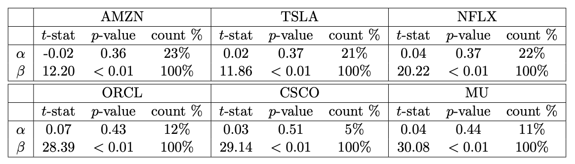
**Predictive power of order flow imbalance.** The orde flow imbalance value was used as the input to a regression model of future price moves. Six stock were used, Amazon (AMZN), Tesla (TSLA), Netflix (NFLX), Oracle (ORCL), Cisco (CSCO), and Micron (MU). The fitted intercept is given by $\alpha$ and the fitted coefficient for the OFI input is $\beta$. In all six cases, the significant was lower than 1% showing that OFI contains information on future price moves.

The OFI value calculated above looks at the best bid and ask. The authors in ⁴ also calculated values for top 5 best prices giving 5 inputs instead of just 1. They found that looking deeper into the order book adds new information on future price moves.

Summary

Here I’ve summarised the key insights from a few papers looking at order volume in a limit order book. The papers show that the order book contains information that is highly predictive of future price moves. But, these moves do not over-come the bid/ask spread.

I’ve added links to the papers in the reference section. Go check them out for more details.

Like what you see? Follow Adrian on Twitter to be notified of new content. Follow

Footnotes

References & Notes

Álvaro Cartea, Ryan Francis Donnelly, and Sebastian Jaimungal: “Enhancing Trading Strategies with Order Book Signals” Applied Mathematical Finance 25(1) pp. 1–35 (2018) ↩︎ ↩︎
Alexander Lipton, Umberto Pesavento, and Michael G Sotiropoulos: “Trade arrival dynamics and quote imbalance in a limit order book” arXiv (2013) ↩︎ ↩︎
Álvaro Cartea, Sebastian Jaimungal, and J. Penalva: “Algorithmic and high-frequency trading.” Cambridge University Press ↩︎
Ke Xu, Martin D. Gould, and Sam D. Howison: “Multi-Level Order-Flow Imbalance in a Limit Order Book” arXiv (2019) ↩︎ ↩︎ ↩︎

Corrections

If you see any mistakes or room for improvement, please reach out to me on Twitter @DrAdrian.

Citation

Please cite this work as:

Letchford (2023), "Key insights: Imbalance in the order book", OS Quant.

In BibTeX please use:

@article{Letchford2023,
    author = {Letchford, Adrian},
    title = {Key insights: Imbalance in the order book},
    journal = {OS Quant},
    year = {2023},
    note = {https://osquant.com/papers/key-insights-limit-order-book/},
}

Interval	Label
\(-1 \geq \rho_t \gt -\frac{1}{3} \)	Sell-heavy
\(-\frac{1}{3} \geq \rho_t \geq \frac{1}{3} \)	Neutral
\(\frac{1}{3} \gt \rho_t \geq 1 \)	Buy-heavy