Interest rates are not necessarily a pure random walk. This assumption falls out from noticing that yields of different bond maturities must be in some way related. Have a look at the yields of the 30 year and 3 year U.S. Treasuries in the plot below. Notice that the 3 year yield bounces up and down mostly below the 30 year yield.
The yields across different maturities is referred to as a yield curve. Yield curve models can get complicated with the need to parameterise the various shapes that the curve can have. However, in this post, we’re going to focus on modelling the two yields in the above chart; a short term rate and a long term rate. Rather than trying to model the exact interest rates, we’re going to model the spread between them as a mean reverting process.
Once we have this mean reverting process, we’ll derive the expected rates, their variances and covariance and calculate the expected return and variances of ETFs that hold bonds of similar maturities.
Interest rate model
We’re going to create a model of the long term interest rate \(r_l(t)\) and the spread between the long term rate and the short term rate \(s(t) = r_l(t) - r_s(t)\). We’ll combine these to create a model of the short term rate \(r_s(t)\). We’ll use an Ornstein—Uhlenbeck process for the spread. This is a type of Vasicek model known as a two-factor equilibrium Vasicek model .
We want to make as few assumptions as possible about the underlying interest rate. We will model the interest rate of the long term bond \(r_l(t)\) as Brownian motion and the spread \(r_s(t)\) as a mean reverting Ornstein—Uhlenbeck process that is uncorrelated to the long term rate:
$$
\begin{aligned}
d r_l(t) &= \sigma_l dW_l(t) \\
d s(t) &= \theta_s (\mu_s - s(t))dt + \sigma_s dW_s(t) \\
E[dW_l(t)dW_s(t)] &= 0 \\
\end{aligned}
$$
Which means that these processes have normally distributed increments. The conditional moments of the long term rates are:
$$
\begin{aligned}
E[r_l(t) | r_l(0)] &= r_l(0) \\
\text{var}[r_l(t) | r_l(0)] &= \sigma_l^2 t \\
\end{aligned}
$$
and the conditional moments of the spread are :
$$
\begin{aligned}
E[s(t) | s(0)] &= s(0) e^{-\theta_s t} + \mu_s(1 - e^{-\theta_s t}) \\
\text{var}[s(t) | s(0)] &= \frac{\sigma_s^2}{2 \theta_s}(1 - e^{-2\theta_s t}) \\
\end{aligned}
$$
Based on the definition of the spread \(s(t) = r_l(t) - r_s(t)\) the short term rate is:
$$
r_s(t) = r_l(t) - s(t)
$$
Which gives us the moments of the short term rates as functions of the long term rate and spread:
$$
\begin{aligned}
E[r_s(t)|r_s(0)] &= E[r_l(t) | r_l(0)] - E[s(t) | s(0)] \\
& = r_l(0) - s(0) e^{-\theta_s t} - \mu_s(1 - e^{-\theta_s t}) \\
\end{aligned}
$$
$$
\begin{aligned}
\text{var}[r_s(t)|r_s(0)] &= \text{var}[r_l(t) | r_l(0)] + \text{var}[s(t) | s(0)] \\
& = \sigma_l^2 t + \frac{\sigma_l^2}{2 \theta_s}(1 - e^{-2\theta_s t}) \\
\end{aligned}
$$
The covariance between the long and short term rate is:
$$
\begin{aligned}
\text{cov}(r_l(t), r_s(t) | r_l(0), r_s(0)) &=
[1, -1]
\left[\begin{matrix}
\text{var}[r_l(t) | r_l(0)] & 0 \\
0 & \text{var}[s(t) | s(0)] \\
\end{matrix}\right]
\left[\begin{matrix}
1 \\
0 \\
\end{matrix}\right] \\
&= \text{var}[r_l(t) | r_l(0)] \\
\end{aligned}
$$
You can play with the model here:
Estimating parameters
We need to estimate the parameters \(\sigma_l\), \(\mu_s\), \(\theta_s\) and \(\sigma_s\).
The volatility of the long rate \(\sigma_l\) can be done with an EWA of the squared changes in the long rate.
For the parameters of the Ornstien-Uhlenbeck process for the spread, we’ll refer to the unconditional moments as given by :
$$
\begin{aligned}
E[s(t)] &= \mu_s \\
\text{var}[s(t)] &= \frac{\sigma_s^2}{2\theta_s} \\
\text{cov}[s(t), s(i)] &= \frac{\sigma_s^2}{2\theta_s} e^{-\theta_s|t-i|}
\end{aligned}
$$
We can use an EWA to estimate these moments and then solve the equations giving us:
$$
\begin{aligned}
\mu_s &= E[s(t)] \\
\theta_s &= \log(\frac{\text{var}[s(t)]}{\text{cov}[s(t), s(t-1)]}) \\
\sigma_s &= \sqrt{2 \theta_s \text{var}[s(t)]} \\
\end{aligned}
$$
If the same half-life is used for all parameters, then this becomes a single parameter model. For a reasonable estimate of what the half-life should be, you can use the method from a previous paper Estimating the half-life of a time series.
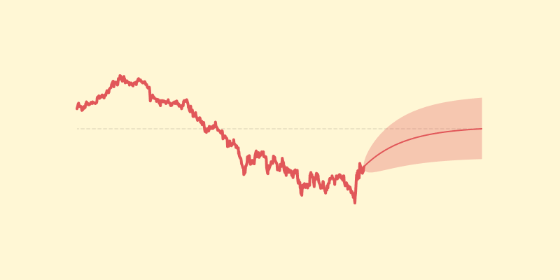
You can see the estimated values for the four parameters here:
ETF Model
We now have a model of the long bond yields and a model of the short bond yields. The next step is to create a model of future ETF returns so that we can trade.
I’m going to refer to a previous article Calculating the mean and variance of bond returns. There I derived the second order Taylor expansion of bond ETF returns as a function of yield and estimated their mean and variance.
The mean is:
$$
E[R_2(r_t)] = C_0 + C_1 E[r_t] + C_2 E[r_t^2]
$$
And the variance is:
$$
\begin{aligned}
\text{var}[R_2(r_t)] &= E[R_2(r_t)^2] - E[R_2(r_t)]^2 \\
\\
E[R_2(r_t)^2] &= C_0^2 + 2C_0C_1E[r_t] + (2C_0 C_2 + C_1^2 )E[r_t^2] \\
&\quad + 2C_1C_2 E[r_t^3] + C_2^2 E[r_t^4] \\
\end{aligned}
$$
Where \(R_2(r_t)\) is the estimated ETF return and \(r_t\) is the bond yield at time \(t\). The \(C_i\) values are functions of the previous period’s bond yield \(r_{t-1}\), the frequency of the yields \(f\), the number of coupons paid per year \(p\) and the time to expiration in years \(T\).
The equations for the \(C_i\) values are a little long and tedious. Their value is that they create a polynomial of the ETF returns as a function of \(r_t\). This makes estimating moments simpler. You can refer to the article if you’re interested in their derivation.
The moments of the yield \(r_t\) are all Gaussian moments which means we can calculate the mean and variance above given the parameters below:
| ETF |
Rates |
Maturity \(T\) |
Frequency \(f\) |
Coupons \(p\) |
| TLT |
DGS30 |
25 |
260 |
2 |
| SHY |
DGS3 |
2 |
270 |
2 |
Here I plot the expected 1-step ahead returns for TLT and SHY:
Simple trading
To test out this model, I made a simple mean variance optimisation to find weights that create a spread. That is, the weights sum to zero. I assume that there are zero trading costs, trading happens at the mid price and the correlation between the ETFs is 1.
Here are the results compared with an equally weighted portfolio:
Straight away, without any parameter tuning we can get better positions in the two ETFs. Comparing against both an equally weighted portfolio and buying and holding TLT, the Sharpe ratio is higher and the drawdowns are lower:
| Strategy |
Sharpe |
Drawdown |
| Buy and hold TLT |
0.41 |
-44.14% |
| Equal positions |
0.50 |
-26.85% |
| TLT & SHY spread |
0.53 |
-18.96% |
These results show that you can model fairly sophisticated interest rate behaviour and take on position with ETFs.